Deterministic ADVI in JAX
This post is about variational inference, and a particular form of automatic differentiation variational inference (ADVI). If you haven’t come across variational inference before, it’s actually quite a simple idea. In Bayesian inference, what we do is specify the prior probability of our parameters, \(p(\theta)\) and a likelihood of the parameters given the data \(y\), \(p(y | \theta)\). The goal is to find the conditional distribution \(p(\theta | y)\) which represents our updated belief about \(\theta\) now that we’ve observed the data \(y\). Bayes’ rule tells us how to do this:
\[p(\theta | y) = \frac{p(\theta) p(y | \theta)}{p(y)}\]Pretty simple so far. One key issue here however is the denominator. \(p(y) = \int p(\theta^*) p(y | \theta^*) d\theta^*\) is something we could compute in principle, but in practice it’s an integral over all elements of \(\theta\), which is hard to compute.
Probably the most popular way out of this problem is Markov Chain Monte Carlo (MCMC). The idea there, very briefly, is to cleverly construct a Markov Chain whose stationary distribution is equal to \(p(\theta | y)\). Amazingly, this isn’t that hard to do, although state-of-the-art MCMC algorithms, such as HMC with NUTS, are quite involved.
MCMC is great. It’s asymptotically exact, meaning that if we run the chain long enough, we should get samples from the posterior distribution \(p(\theta | y)\). Unfortunately, this can take a long time. Software packages like Stan draw thousands of samples, and each draw involves multiple (likely tens, perhaps hundreds) of evaluations of the un-normalised log posterior, \(\log p(\theta) + \log p(y | \theta)\). This is fine for many models, but sometimes it just takes too long.
What’s variational inference?
Variational inference is another way to do Bayesian inference. Here, the idea is that we’ll approximate the posterior distribution with a family of distributions that is easy to work with. One popular such family is the mean-field family of distributions:
\[q(\theta; \eta) = \prod_{k=1}^K q(\theta_k ; \eta_k)\]The notation here says that we are introducing a distribution \(q(\theta; \eta)\) over \(\theta\) parameterised by \(\eta_k\), the “variational parameters”. The mean-field approximation means that we’re breaking the parameters \(\theta\) into \(K\) groups, each of which is modelled as independent from all of the other groups. The particular approximating family in this post is the mean field family consisting of univariate normal distributions:
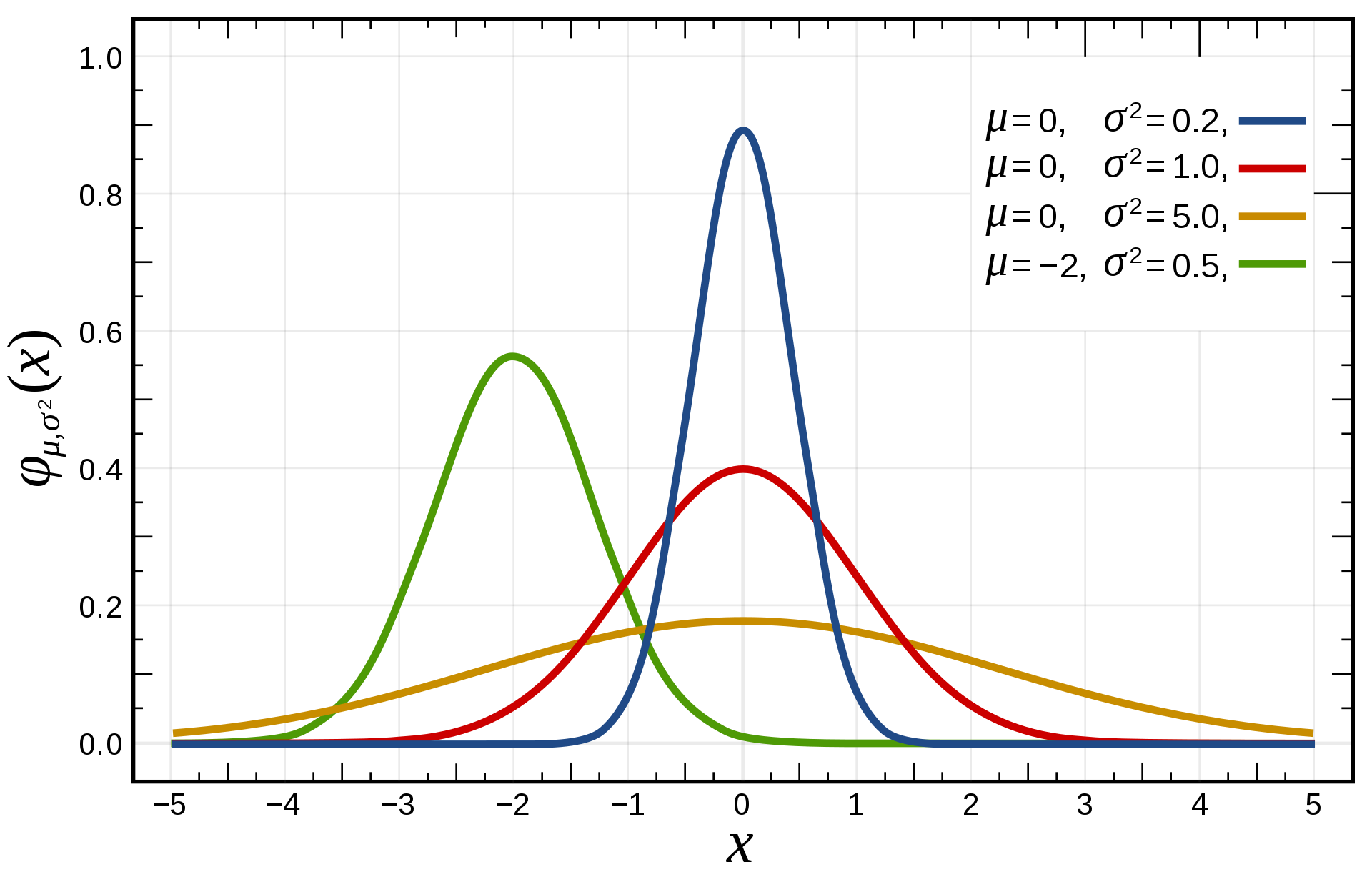
\[q(\theta; \eta) = \prod_{k=1}^K \mathcal{N}(\theta_k | \mu_k, \sigma_k^2)\]Here, the variational parameters \(\eta\) are the set of means and variances, \(\mu_k\) and \(\sigma_k^2\), for each of the elements of vector of parameters \(\theta\).
The idea in variational inference is to find an optimal set of parameters, \(\eta^* = \{\mu_1^*, ... \mu_K^*, \sigma^{2*}_1, ... \sigma^{*2}_K\}\) in such a way that the distribution \(q(\theta; \eta^*)\) is as close to the actual posterior \(p(\theta | y)\) as possible. We do this by minimising a discrepancy measure between the true posterior and the approximating distribution. There are many possible choices, but the usual one is the Kullback-Leibler divergence between \(q(\theta; \eta)\) and \(p(\theta | y)\), defined as:
\[\textrm{KL}[q(\theta; \eta) || p(\theta | y)] = \mathbb{E}_{q(\theta; \eta)} \log \frac{q(\theta ; \eta)}{p(\theta | y)}\]The notation with the subscript means that the expectation is taken over the variational distribution \(q(\theta; \eta)\). Why this discrepancy measure? The short answer is that it’s easy to work with. In general, it has some properties that are good, such as that it’s zero when the two distributions are identical, and it’s positive otherwise. However, it’s not ideal in some ways. For example, it’s not symmetric: \(\textrm{KL}[q || p] \neq \textrm{KL}[p || q]\). This means it’s not technically a distance. It also tends to favour approximations that underestimate the variance. In general, minimising the KL divergence will result in approximate distributions that get the means right but underestimate the variance. That’s hardly ideal, but in cases where MCMC would be too slow, it can still provide useful inference.
What’s ADVI?
Assuming we’re on board with approximating the posterior using a chosen family of distributions, there’s still the issue of how we can actually do that. In the past, this was anything but easy. Just look at the variational inference section of Chris Bishop’s excellent book. The “old-school” approach relies on the fact that, if the mean-field approximation is made, a coordinate-ascent procedure to minimize the KL divergence can be derived. The updates in this procedure take the form of expectations which can be calculated in closed form for some models. There’s absolutely nothing wrong with this approach, except that it can involve a lot of calculations, and that it can only be applied to a certain subset of models.
Automatic differentiation variational inference promises to do black-box variational inference instead. Here, black-box means that we don’t have to know any details about \(p(\theta | y)\); any model for which we can evaluate (and differentiate) the log likelihood and log prior distributions will do. That’s a big difference compared to the coordinate-ascent VI described in the previous paragraph. To see how it works, let’s first write out the KL divergence again:
\[\textrm{KL}[q(\theta;\eta) || p(\theta | y)] = \mathbb{E}_{q(\theta;\eta)} [\log q(\theta; \eta) - \log p(\theta|y)]\]There are two terms on the right hand side. The first is:
\[\mathbb{E}_{q(\theta;\eta)}[\log q(\theta; \eta)]\]You might recognise this as the negative entropy \(S\) of the distribution \(q(\theta; \eta)\). We are free to choose the variational distribution, so we can choose it in a way that allows us to compute this term. For example, if we use a factorising normal distribution as our approximation, the negative entropy is:
\[\mathbb{E}_{q(\theta;\eta)}[\log q(\theta; \eta)] = -S(\eta) = -\sum_k\log(\sigma_k) + constant,\]where the sum ranges over the individual elements of the vector \(\theta\).
The second term is:
\[\mathbb{E}_{q(\theta;\eta)}[-\log p(\theta| y)]\]This is the expectation of the negative log posterior under the variational approximation. However, the whole point of inference is that we don’t know the log posterior distribution! Using Bayes’ rule, we can rewrite \(\log p(\theta|y)\) as:
\[\log p(\theta | y) = \log p(\theta) + \log p(y | \theta) - \log p(y)\]When we take the expectation, we see that the final term, \(\log p(y)\), does not depend on \(\theta\) and is therefore a constant. So we can simplify the objective to:
\[\textrm{KL}[q(\theta;\eta) || p(\theta | y)] = - S(\eta) - \mathbb{E}_{q(\theta;\eta)} [\log p(\theta) + \log p(y | \theta)] + constant\]That’s better. We can evaluate \(p(\theta)\) – that’s just the prior – and we can evaluate \(p(y | \theta)\) – the likelihood. This way of carving up the \(\textrm{KL}\) divergence also has a nice interpretation: we simulatenously want to maximise the entropy of the approximating distribution (by minimising \(-S(\eta)\)) while also maximising the expected log joint distribution of \(\theta\) and \(y\) (by minimising the second and third terms), which will be high if the data are fit well and we are close to the prior.
That’s nice, but we’re still left with having to calculate the expectations of the two terms \(\log p(\theta)\) and \(\log p(y | \theta)\). Sometimes this can be done analytically, and sometimes we can do it efficiently with something called Gauss-Hermite quadrature, which is almost as good. In Gaussian Processes for example, this works really well. But that’s for another blog post to cover.
ADVI does this differently. To understand how, let’s first consider taking the gradient of the KL divergence so that we can use gradient-based methods to optimise it. Taking the gradient of the expression above with respect to the variational parameters \(\eta\) gives:
\(\nabla_\eta \textrm{KL}[q(\theta;\eta) || p(\theta | y)] = -\nabla_\eta S(\eta) - \nabla_{\eta} \mathbb{E}_{q(\theta;\eta)} [\log p(\theta) + \log p(y | \theta)]\).
You might think that you could exchange the expectation and gradient operators and estimate this by Monte Carlo expectation: first sample a \(\theta\) from \(q(\theta; \eta)\) using the current parameters \(\eta\), then use automatic differentiation to compute the gradient of the terms in the expectation. However, that would ignore that the expectation itself is taken over \(q(\theta; \eta)\), which depends on \(\eta\)!
It’s actually possible to derive an estimator of the gradient, and it’s not that hard (see the BBVI paper). I haven’t tried it, but it’s generally described as suffering from high variance, meaning that you would need a lot of Monte Carlo samples to get a good estimate of the gradient. Thankfully, for some approximating distributions, we can use something called the “reparameterisation trick” instead. If our approximating distribution is a factorised normal distribution, we can draw samples from it by doing the following:
\(z_i \sim \mathcal{N}(0, 1)\),
\(\theta_i = \mu_i + \sigma_i z_i\),
and \(\theta_i\) will have a \(\mathcal{N}(\mu_i, \sigma_i^2)\) distribution. We can use this trick to rewrite the expectation:
\(\mathbb{E}_{q(\theta; \eta)}[f(\theta)] = \mathbb{E}_{p(z)}[f(\theta(z))]\),
where \(f(\theta) = \log p(\theta) + \log p(y | \theta)\). This is a valid thing to do thanks to the law of the unconscious statistician. Now, the expectation is no longer taken over the variational parameters, and we can exchange the gradient and expectation operators. We are left with:
\[\nabla_\eta \textrm{KL}[q(\theta;\eta) || p(\theta | y)] = -\nabla_\eta S(\eta) - \mathbb{E}_{p(z)}[ \nabla_{\eta} [\log p(\theta(z)) + \log p(y | \theta(z))]]\]Great! Now we can do a Monte Carlo expectation. At each step, draw some samples \(z\), compute \(\theta(z)\) for each, calculate \(\log p(\theta(z)) + \log p(y | \theta(z))\), for each, take the mean, and use autodiff to get the gradients.
This is basically how ADVI works. There’s one more component: because the approximating distribution and the target distribution have to have the same support, any parameters that have limited support have to be transformed to lie in unconstrained space for the normal distributions to be a valid approximating distribution. For example, variance parameters take values between 0 and \(+\infty\), and a \(\log\) transformation maps them to be between \(-\infty\) and \(+\infty\). This complicates things a little bit, but not a great deal.
In the original paper, the objective is optimised using stochastic optimisation. Stochastic optimisers such as Adam and RMSProp are popular in deep learning, and they definitely have advantages. One nice thing is that we can just use minibatches and scale to problems that wouldn’t fit into memory. This is probably essential for models like deep neural nets where it would be hopeless to try to use the whole dataset. However, stochastic optimisation has issues which I’d like to talk about in the next section.
The problem with ADVI
ADVI sounds great in principle. It has limitations, of course. The mean-field approximation will underestimate the posterior variance, but it will tend to at least get the means of the parameters correct. Full MCMC is preferable when possible, but for very large-scale models where it isn’t an option, ADVI sounds like a good alternative.
There’s a catch though: stochastic optimisation. As anyone who’s played with neural nets can probably tell you, getting stochastic optimisers to work properly can be extremely fiddly. It’s not clear how the step size should be chosen, and even the adaptive algorithms like the one proposed in the ADVI paper have free parameters that have to be set. Stan has a scheme that tries to set them intelligently, but it can go wrong. It’s also not easy to be sure of convergence. I’ve generally avoided ADVI for that reason and generally preferred other ways to approach variational inference, especially the GP approach I mentioned earlier, which can be used with approximate second-order methods like L-BFGS.
A possible fix: “Deterministic” ADVI
At this year’s StanCon, I had a chat with Ryan Giordano, who presented some really cool work on frequentist covariances of posterior expectations. He mentioned that when he worked with ADVI, rather than making a new draw \(z\) at each step of the optimisation, which means that we have to use stochastic optimisers, he preferred to make a single set of draws at the start and keep them fixed during the optimisation. He talks about this and justifies it in a great paper, Covariances, Robustness, and Variational Bayes, written with Tamara Broderick and Michael I. Jordan. The focus of the paper is on a method to improve the covariance estimates made by variational inference, but I think the idea of fixing the draws should receive more attention in its own right.
Why is it such a big deal? In short, the great thing about fixing the draws is that the stochasticity in the objective is gone: conditional on the draws \(z\), the objective is deterministic. That means we can use approximate second-order methods like L-BFGS. Giordano et al. actually use full second order methods which require the calculation of Hessian vector products. They write that these are essential for their method of improving covariance estimates since they find the optimum of the objective more precisely. I’ve found L-BFGS to work fine for “vanilla” ADVI though (at least so far). What’s so cool in my opinion is that L-BFGS is much less fiddly than stochastic optimisation. It “just works” – there are no tuning parameters.
Implementation in JAX
People who follow me on Twitter will likely know that I am a huge fan of the python library JAX. It turns out it was really easy to implement the deterministic variant of ADVI in JAX. I’ve put together a simple interface which allows you to fit Bayesian models with it. Here’s how you would code up a simple logistic regression:
\[\mathbf{f} = \mathbf{X} \pmb{\beta} + \gamma\] \[\mathbf{y} \sim \textrm{Bern}(\textrm{logit}^{-1}(\mathbf{f}))\] \[\pmb{\beta} \stackrel{iid}{\sim} \mathcal{N}(0, 1)\] \[\gamma \sim \mathcal{N}(0, 1)\]from jax_advi.advi import optimize_advi_mean_field
from jax import jit
from jax.scipy.stats import norm
from functools import partial
from jax.nn import log_sigmoid
# Define parameter shapes:
theta_shapes = {
'beta': (K),
'gamma': ()
}
# Define a function to calculate the log likelihood
def calculate_likelihood(theta, X, y):
logit_prob = X @ theta['beta'] + theta['gamma']
prob_pres = log_sigmoid(logit_prob)
prob_abs = log_sigmoid(-logit_prob)
return jnp.sum(y * prob_pres + (1 - y) * prob_abs)
# Define a function to calculate the log prior
def calculate_prior(theta):
beta_prior = jnp.sum(norm.logpdf(theta['beta']))
gamma_prior = jnp.sum(norm.logpdf(theta['gamma']))
return beta_prior + gamma_prior
# The partial application basically conditions on the data (not defined in this
# little snippet)
log_lik_fun = jit(partial(calculate_likelihood, X=X, y=y))
log_prior_fun = jit(calculate_prior)
# Call the optimisation function
result = optimize_advi_mean_field(theta_shapes, log_prior_fun, log_lik_fun, n_draws=None)
And there you go! You just define a likelihood function, a prior function, and the shapes of the parameters. The single function does the rest. If you want to try it for yourself, there are instructions and more examples in the repository.
I ran this simple example and compared the estimates to Stan. With some random data (1000 examples, 10 covariates), here’s a comparison of the posterior means and standard deviations of $\pmb{\beta}$:
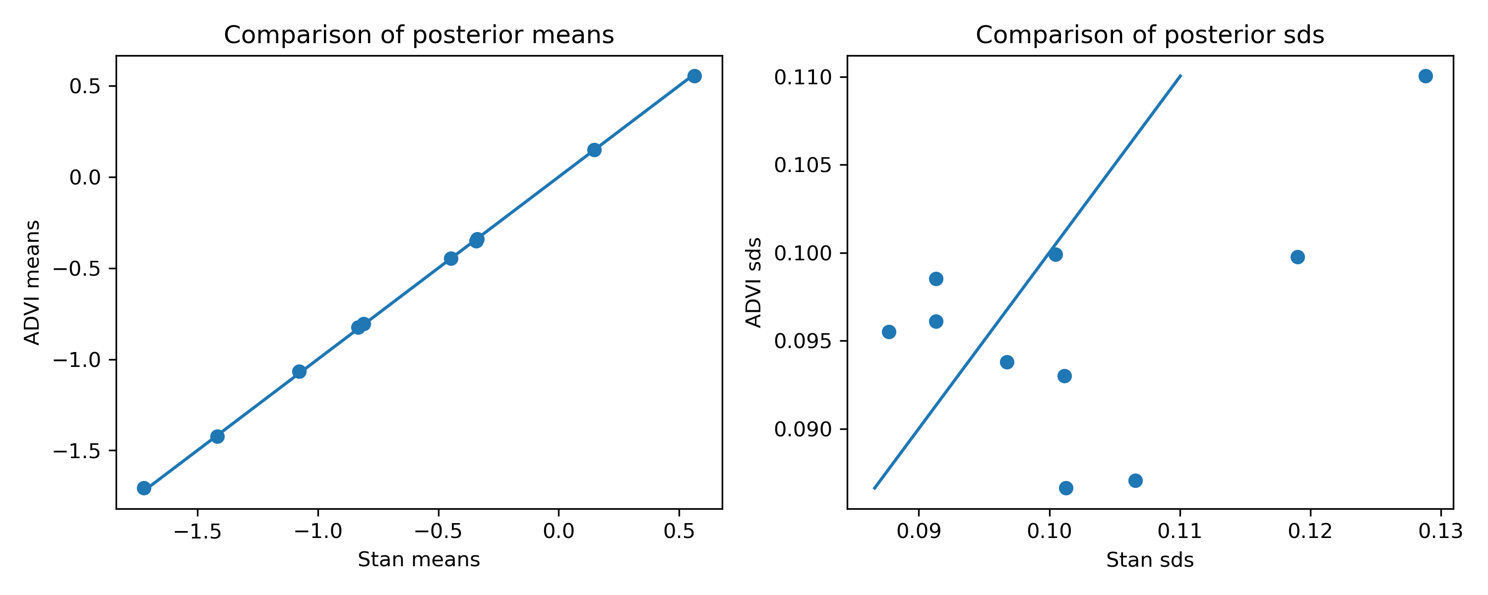
You can see that the means are very good, but the standard deviations are a bit off. I’m actually a bit surprised that the ADVI estimates are not all underestimates. You can see that they are roughly in the right ballpark, but not quite right.
A second example: tennis ratings for the Open Era
ADVI works fairly well on that toy example, but of course it’s extremely contrived. If you want to do logistic regression, MCMC is probably fast enough, and when it isn’t, you likely have enough data to just use maximum likelihood. So here’s another model where ADVI is more useful.
The model is a hierarchical Bradley-Terry model to rate tennis players. That sounds a little fancy perhaps but it’s actually quite a simple model:
\[y_i \sim \textrm{Bernoulli}(p_i)\] \[p_{i} = \textrm{logit}^{-1}(\alpha_{w[i]} - \alpha_{l[i]})\] \[\alpha \stackrel{iid}{\sim} \mathcal{N}(0, \sigma_{\alpha}^2)\] \[\sigma_{\alpha} \sim \mathcal{N}(0, 1)\]where $w[i]$ and $l[i]$ are the winners and losers in match $i$. Writing the data like this in terms of the winner and loser implies that $y_i$ is just a vector of ones. The idea in this model is that each player has a latent skill $\alpha$ drawn from the population distribution. When two players meet, the probability of player $m$ beating player $n$ is given by the difference in their skill, transformed by the inverse logit function.
What makes this model a bit tricky to fit is that it’s hierarchical: we want to estimate $\sigma_\alpha$ and the $\alpha$s together. That makes inference a bit tricky: for example, just finding the posterior mode would likely fail to give a good estimate of $\sigma_\alpha^2$.
The full dataset contains 158,394 matches played between 4,763 players, so it’s
fairly large. Using jax_advi, we can code it as follows. First, define the
shapes:
theta_shapes = {
    'player_skills': (n_p),
    'skill_prior_sd': ()
}
Where n_p is the number of players. I’ve given $\alpha$ the more descriptive
name player_skills and similarly $\sigma_\alpha$ is referred to as
skill_prior_sd.
Here’s something new: we need to constrain the prior sd to lie between 0 and $+\infty$. We can do this as follows:
from jax_advi.constraints import constrain_positive

theta_constraints = {
    'skill_prior_sd': constrain_positive
}
The constraint function will ensure that we correct for the transformation when computing the prior density. Now we define our prior and log likelihood:
from jax.scipy.stats import norm
from jax import jit
from jax.nn import log_sigmoid
import jax.numpy as jnp

@jit
def log_prior_fun(theta):

    # Prior
    skill_prior = jnp.sum(norm.logpdf(theta['player_skills'], 0., theta['skill_prior_sd']))

    # hyperpriors
    hyper_sd = norm.logpdf(theta['skill_prior_sd'])

    return skill_prior + hyper_sd

def log_lik_fun(theta, winner_ids, loser_ids):

    logit_probs = theta['player_skills'][winner_ids] - theta['player_skills'][loser_ids]

    return jnp.sum(log_sigmoid(logit_probs))

from functools import partial

curried_lik = jit(partial(log_lik_fun, winner_ids=winner_ids, loser_ids=loser_ids))
And finally, we can fit the model:
result = optimize_advi_mean_field(
	theta_shapes, log_prior_fun, curried_lik,
	constrain_fun_dict=theta_constraints, verbose=True, M=100)
Here are the timings on my laptop with a GeForce GTX 2070: 9.43 s ± 456 ms per loop (mean ± std. dev. of 7 runs, 1 loop each)
Stan can fit this model too, it just takes much longer. For this model, it took around 100 minutes. That means I’d really still suggest using Stan for this model, but if we start to make things more complicated (e.g. adding surface effects), it might get very slow. Or you could prototype your model with ADVI and then use Stan or another MCMC package like greta when you want to get good variance and covariance estimates.
How do the estimates compare?
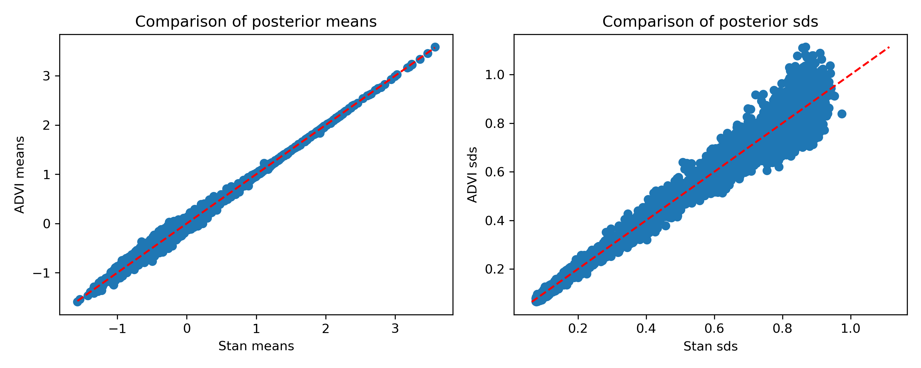
Once again, the means are pretty good, and the standard deviations aren’t terrible but are definitely slightly off. Again I’m a bit surprised they’re not all smaller than Stan’s, but that’s how things are looking.
How about Stan’s (stochastic) ADVI implementation? Here it is compared against HMC’s result:
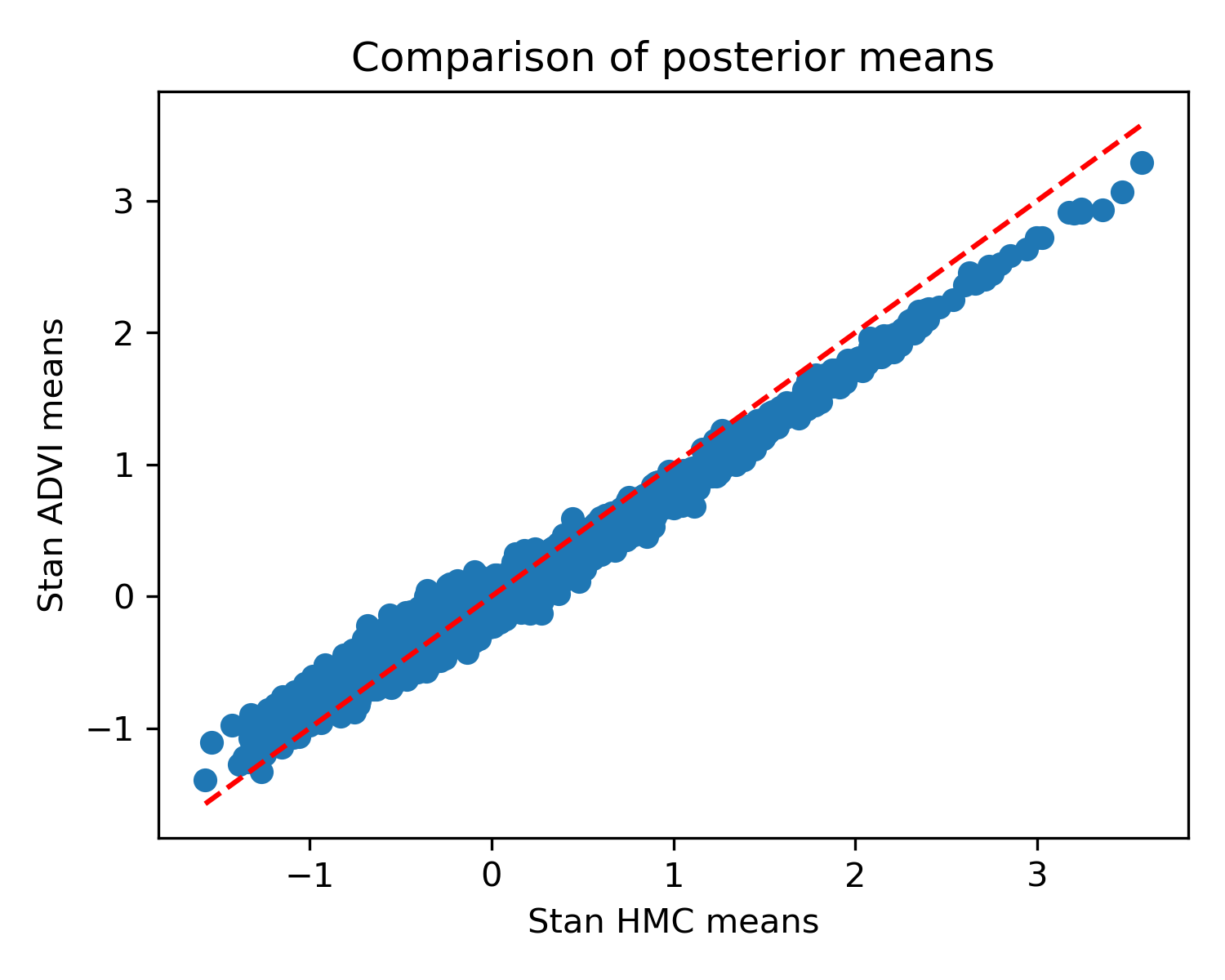
You can see that it’s not terrible, but unlike the determinstic version, the means are a bit off. I didn’t see a quick way to extract the variances.
Overall, I’m excited about this, and I already have some applications in mind for this variant on ADVI. If you’d like to give my little package a go, please fetch it from its repository. I hope you find it useful.
This has been quite a technical post, but to have a little bit of tennis in it, I’ll leave you with the ten players with the highest mean ratings:
| Rating | |
|---|---|
| Novak Djokovic | 3.58 |
| Rafael Nadal | 3.45 |
| Roger Federer | 3.34 |
| Ivan Lendl | 3.23 |
| Bjorn Borg | 3.23 |
| John McEnroe | 3.18 |
| Jimmy Connors | 3.16 |
| Rod Laver | 3.03 |
| Andy Murray | 2.99 |
| Pete Sampras | 2.92 |