If you like sports analytics, chances are you have come across the Elo rating system. The idea behind it is simple. Every player starts with a rating of 1500. When two players meet, the probability that player A beats player B is given by:

Let’s say A does end up winning. Then, to make an update, we calculate a residual $r$:

and update A and B’s Elo ratings as follows:

where $k$ is a constant, often set to 32. That’s it! We just iterate this process, updating each player’s rating based on their results using the formulae above.

What I’ve been thinking about lately is the problem that the optimal $k$ may change over time, and what that might mean. It turns out that if you take a Bayesian point of view, $k$ can be related to the prior variance of player skills (see for example, Mark Glickman’s Glicko paper, equation 13, and I’ll have a paper with some thoughts about this out soon too). Basically, the more uncertain we are about competitors’ skill levels, the larger $k$ is going to be.

I think it’s worth thinking about this a bit more. This is still quite speculative, but I wonder whether, if we could fit a model that estimates time-varying $k$ factors, it might tell us something about the depth of competition in that period. The reasoning is that if a large $k$ implies a large prior variance, that means that the average (absolute) difference in ratings between two random players is going to be greater when $k$ is large. This may be obvious, but just in case, here’s an example: let’s say the prior is normal with a standard deviation of 100. A simulation suggests that the absolute difference in ratings between two random players is, on average, about 113. On the other hand, if the prior standard deviation is 50, that difference drops to 56. So any given match is likely to be closer in the second case.

What this suggests is that, if we have a large $k$ in a given period, we might conclude that this period is slightly less competitive than others. It would also make high Elo ratings in that period more likely, as a player would need fewer victories to increase their rating.

To investigate this idea a bit, I fit a model in Stan that estimates a time-varying $k$-factor using a random walk on $k$. The random walk bit just encodes the idea that $k$ is unlikely to vary dramatically from one year to the next; instead, it’s a small random step up or down. Here are the estimates when fit to ATP data since 1969:

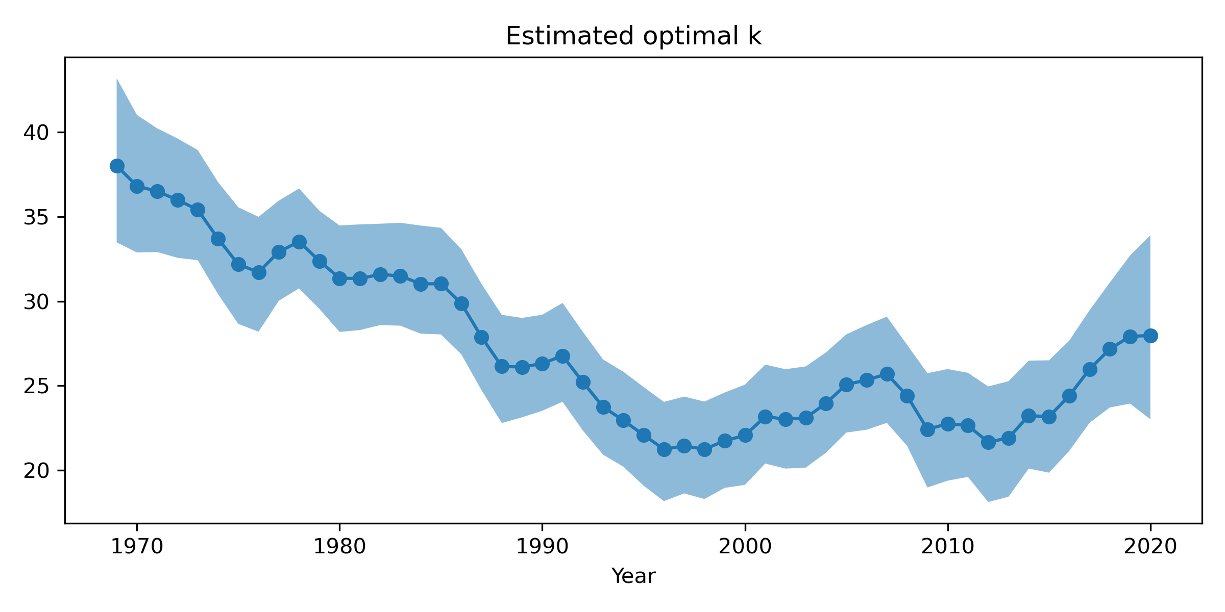
Although I can’t say that I fully understand what is going on here, the trends are quite interesting. $k$ starts off quite large, perhaps implying a large range of skills, and declines until it reaches a low point sometime in the late 90s. There was a bit of a rise in the 2000s, a drop around 2010, and another rise again from about 2015 onwards. It’s intriguing to think about possible causes of the changes that are observed. For example, what about that sharp drop from 1985 - 1988? Or the second drop from 1991-1996? I can’t help but wonder whether playing equipment played a role here – certainly players switched from wood to graphite around the mid-80s, so maybe that had something to do with the first drop. But of course it’s hard to say, many factors could be at play here.

Another point I think is quite interesting to think about is what this means about peak Elo ratings and how impressive they are. For example, when fitting standard Elo with a fixed $k$, the highest Elo ratings belong to Bjorn Borg (2455, reached in 1980), and John McEnroe (2429, reached in 1985), followed by Novak Djokovic (2423, reached in 2016). But the dynamic $k$ estimates suggest that it was harder to reach this rating in 2016, when $k$ was quite a bit smaller (about 23 for Djokovic compared to about 31 for McEnroe/Borg). A simple way to see this is that $k$ determines the maximum number of points gained from any one victory, so more match wins are needed to reach a given level when $k$ is smaller.

Besides $k$, we might also wonder whether the initial skill of players changed over time. We can fix the initial rating for a new player in 1969 to 1500 and then estimate a similar random walk for the initial skill of a new player since then. This is what we get:

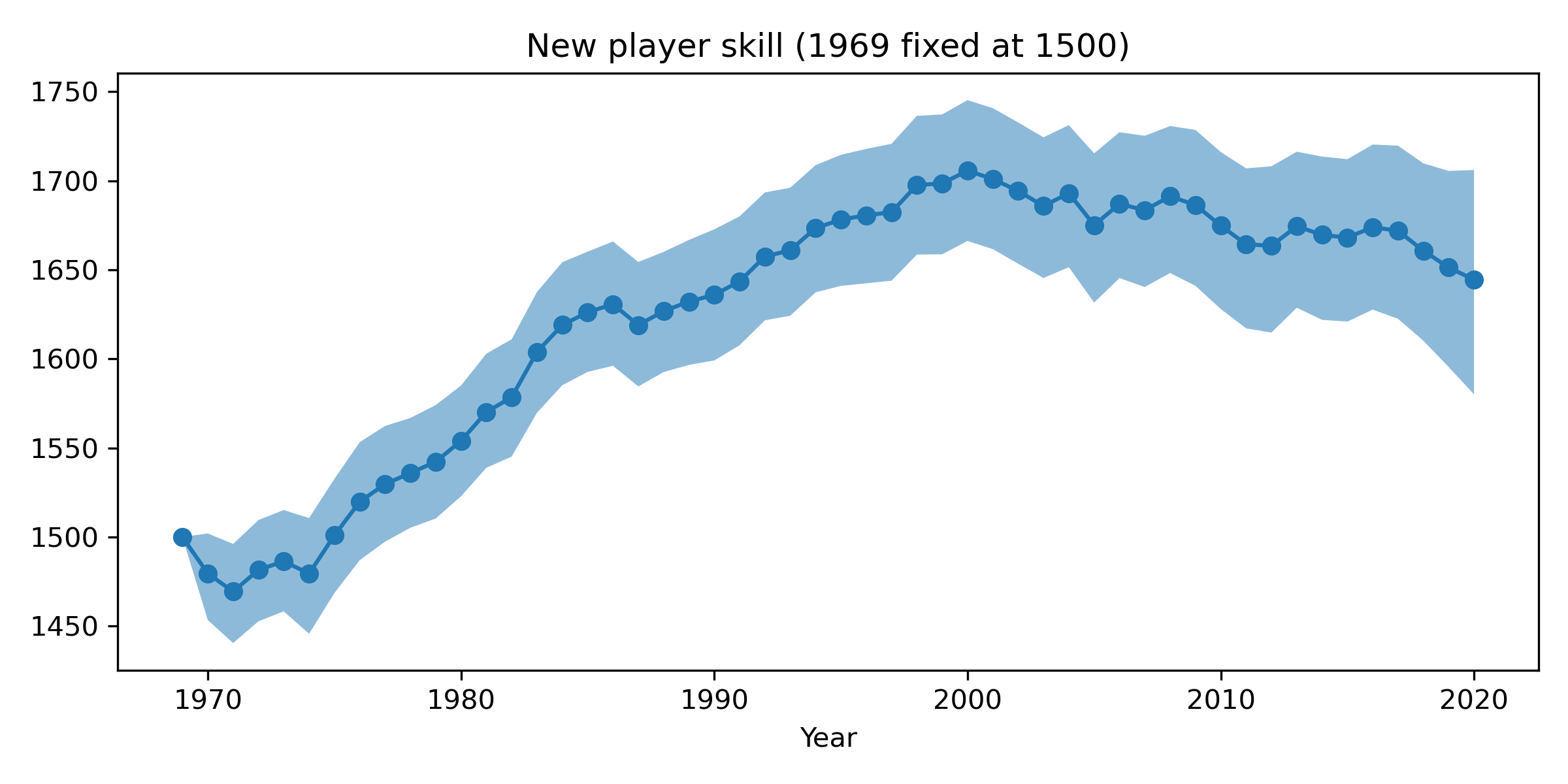
This plot is also pretty intriguing, I think. It looks like new players’ skills started increasing from around 1975, rising pretty much non-stop until around 2000, before levelling off and maybe falling a little bit recently. The figure would imply that a player playing their first match on tour in 1980 would have an Elo rating of about 1550, quite a bit lower than that of a player starting in 2000, whose skill would be around 1700. The trends are consistent with the idea that each generation improves on the previous one, at least until 2000. I’m not sure what explains the plateau since then, and perhaps it’s best not to read too much into it.

Overall, I wanted to share these results even though I can’t say I really understand all their implications just yet. It’s a little bit odd to use Elo as part of a Bayesian model like this, for example, and I need to think about what exactly that means. Overall, though, I do think this idea of fitting time-varying $k$ factors is a good one, and I hope you agree that the results are, if anything, an interesting start.

Stan code

If you’re curious, here’s the Stan code for fitting the model:

data {
  int n_players;
  int n_matches;
  int n_periods;

  int period[n_matches];
  int winner_ids[n_matches];
  int loser_ids[n_matches];
} 
parameters {
  vector<lower=0>[n_periods] ks;
  vector[n_periods - 2] mu_additions;
  real initial_offset;

  real<lower=0> k_time_sd;
  real<lower=0> mu_time_sd;
}
transformed parameters {
  vector[n_periods] mus;
  // The second year is the baseline
  mus[2] = 1500.;

  // First year gets an offset
  mus[1] = 1500. + initial_offset;

  // ... and we have a random walk from then on.
  mus[3:] = mus[2] + cumulative_sum(mu_additions);
}
model {

  vector[n_players] cur_player_skills = rep_vector(-1, n_players);
  int previously_seen[n_players] = rep_array(0, n_players);

  // Priors on the random walk variances
  k_time_sd ~ normal(0, 1);
  mu_time_sd ~ normal(0, 30);

  // Prior on the initial drop
  initial_offset ~ normal(0, 50);

  // Prior for initial k (not part of random walk)
  ks[1] ~ normal(32, 10);

  // Prior for next k
  ks[2] ~ normal(32, 10);

  // Random walk prior on k for the rest:
  for (i in 3:n_periods) {
    ks[i] ~ normal(ks[i - 1], k_time_sd);
  }

  // Random walk prior on mu:
  mu_additions ~ normal(0, mu_time_sd);

  // Now for the likelihood.
  for (i in 1:n_matches) {

    // Check whether they've been previously seen
    int winner_seen = previously_seen[winner_ids[i]];
    int loser_seen = previously_seen[loser_ids[i]];

    // Find their skills
    real cur_winner_elo = (winner_seen == 1) ? cur_player_skills[winner_ids[i]]
					     : mus[period[i]];

    real cur_loser_elo = (loser_seen == 1) ? cur_player_skills[loser_ids[i]]
					     : mus[period[i]];


    // Compute the win probability
    real win_prob = 1 / (1 + pow(10, -(cur_winner_elo - cur_loser_elo) / 400));

    // Update the arrays:
    previously_seen[winner_ids[i]] = 1;
    previously_seen[loser_ids[i]] = 1;

    // Compute the updates
    cur_player_skills[winner_ids[i]] = cur_winner_elo + ks[period[i]] * (1 - win_prob);
    cur_player_skills[loser_ids[i]] = cur_loser_elo + ks[period[i]] * (0 - (1 - win_prob));

    // Add to the log likelihood
    target += log(win_prob);

  }
}