A first model to rate Formula 1 drivers
I wasn’t much of a fan of Formula 1 growing up. However, things have changed! I watched Netflix’s “Drive to Survive” documentary and it did a great job introducing the nuances of the sport. I’m now a big fan and look forward to every race weekend.
Naturally, I started thinking about statistical questions. In particular, I’m fascinated by trying to work out who is actually the best driver in Formula 1. Max Verstappen and Lewis Hamilton are currently winning most of the races. But they are also very likely to have the best cars. It’s well known that cars play a major role in F1, and that makes it incredibly difficult to say who is the best driver.
This short blog post is about some initial work I’ve been doing to try to answer this question. I’m not the first to look at this: there are some interesting papers out on this already (e.g. this one). And, as I’ll talk about, there are some improvements I’d like to make to the simple model I’ve come up with. But it’s a start, its results are fairly reasonable, and I’m interested to hear people’s thoughts.
How can we build a model for F1 prediction? Let’s dive in.
A likelihood for rankings
The first thing to work out, at least for me, was choosing which likelihood to use. This is actually not an easy question to answer! There are many possibilities here: one could use the times, or speeds, for example. Or one could use the point scored in each race. The one that I have initially chosen is based on the finishing position. To do that, I use a rank-ordered logit model. In this model, the probability that driver A finishes ahead of drivers B and C is given by
\[P(\text{A beats B and C}) = \frac{\exp(\theta_A)}{\exp{(\theta_A)} + \exp{(\theta_B)} + \exp (\theta_C)},\]where the $\theta$ are their latent skills. This is a version of a Bradley-Terry-Luce model. Some great resources I found on this model are this document and Mark Glickman’s rank-ordered logit paper.
In Stan, we can write the log likelihood this implies for a larger number of competitors (here given as the argument n_per_race) as:
    real compute_log_likelihood(vector cur_skills, int n_per_race) {

        real cur_lik = 0;

        for (cur_position in 1:(n_per_race - 1)) {
            vector[n_per_race - cur_position + 1] other_skills;

            for (cur_other_position in cur_position:n_per_race) {
                other_skills[cur_other_position - cur_position + 1] = cur_skills[cur_other_position];
            }

            real cur_numerator = cur_skills[cur_position];
            real cur_denominator = log_sum_exp(other_skills);
            cur_lik += cur_numerator - cur_denominator;
        }

        return cur_lik;

    }
This computes the probability above for each driver on the log scale, and then sums them up. The log_sum_exp function makes sure that we don’t have any numerical issues when computing the denominator.
What goes into the skills $\theta$? There are lots of interesting things to consider here, but the simple model I’ve gone for initially is:
\[\theta = \text{driver_skill} + \text{car_skill}.\]To make things a bit more realistic, I assume these are dynamic, i.e. they are allowed to change from year to year. That’s important because we know that teams are constantly trying to improve their cars, and drivers’ skills can change from year to year too. Because we don’t expect car and driver skills to change dramatically from one season to the next, I assume that they follow a random walk. That just means that we assume that on average, skills remain the same from one season to the next, but they could get a little bit better or worse.
Handling DNFs
This is only part of the puzzle though. In F1, “DNFs” are possible, and in fact happen fairly routinely. DNF stands for “did not finish”, and they can be due to driver error (e.g. causing a collision), or mechanical issues. If a driver does not finish, they are ranked last, and if multiple drivers fail to finish, they are ranked by how many laps they completed (if I remember correctly, but this is not crucial here).
Since we do have an assigned ranking even for DNFs, then, we could just use that in the likelihood above. However, I think it is preferable to model DNFs separately (I’ll talk a bit about why later). To do that, I use the rank log likelihood above only for those drivers that finished. To model DNFs, I use a Bernoulli likelihood on a DNF indicator for each driver and race. The model for the probability of a DNF is:
\[\text{logit}(p_{\text{DNF}}) = \text{driver_risk} + \text{car_risk} + \text{intercept},\]so it closely parallels the model for $\theta$. In the future, I think it’ll be useful to not just use a DNF indicator, but to distinguish accidents/collisions (which are likely due to the driver) from mechanical issues (which are likely due to the car). That might make it easier for the model to distinguish the two types of risk.
I assume that car risks also follow a random walk over time, and that the driver risk remains constant throughout the period. The idea here is that cars might become more or less reliable between seasons, but drivers are likely to be relatively stable in their risk preferences.
The advantage of modelling DNFs this way is that we can consider two scenarios: (1) what happens if everyone races without incidents, and (2) how likely it is that someone DNFs. Ignoring DNFs would muddle the two and not allow us to assess team and driver differences among DNFs.
A potential problem
Before diving into the results, I wanted to mention that I am aware of one issue with this model setup: the grey zone between DNFs and regular races. I’ve noticed that some races are assigned a very low log likelihood under the model. One such race is the 2021 Azerbaijan GP in Baku. Now, this was clearly a surprising race – take a look at the finishing order:
| Position | Driver |
|---|---|
| 1 | perez |
| 2 | vettel |
| 3 | gasly |
| 4 | leclerc |
| 5 | norris |
| 6 | alonso |
| 7 | tsunoda |
| 8 | sainz |
| 9 | ricciardo |
| 10 | raikkonen |
| 11 | giovinazzi |
| 12 | bottas |
| 13 | mick_schumacher |
| 14 | mazepin |
| 15 | hamilton |
| 16 | latifi |
| \N | russell |
| \N | max_verstappen |
| \N | stroll |
| \N | ocon |
The drivers with the \N are the DNFs. But even among those that did finish there are some big surprises. For example, Mazepin is ahead of Hamilton! This kind of result is very unlikely under the model. But there is an easy explanation: the race was restarted very late, and Hamilton had a lockup. Clearly then, there is a third type of race between DNFs and finishing: finishing, but with a severe issue or error on the way. It would be great to be able to distinguish these, but I haven’t gone to those lengths yet. I don’t know to what extent this affects the ratings, but I wanted to mention that this might be an issue.
Some results
Now for the fun part: some initial results! Here, I’m using data from 2014 onwards, as I thought it might be good to stay in the current era of racing. This is using the terrific Ergast CSVs which I can highly recommend.
Team ratings
First off, let’s take a look at the mean team ratings over time:
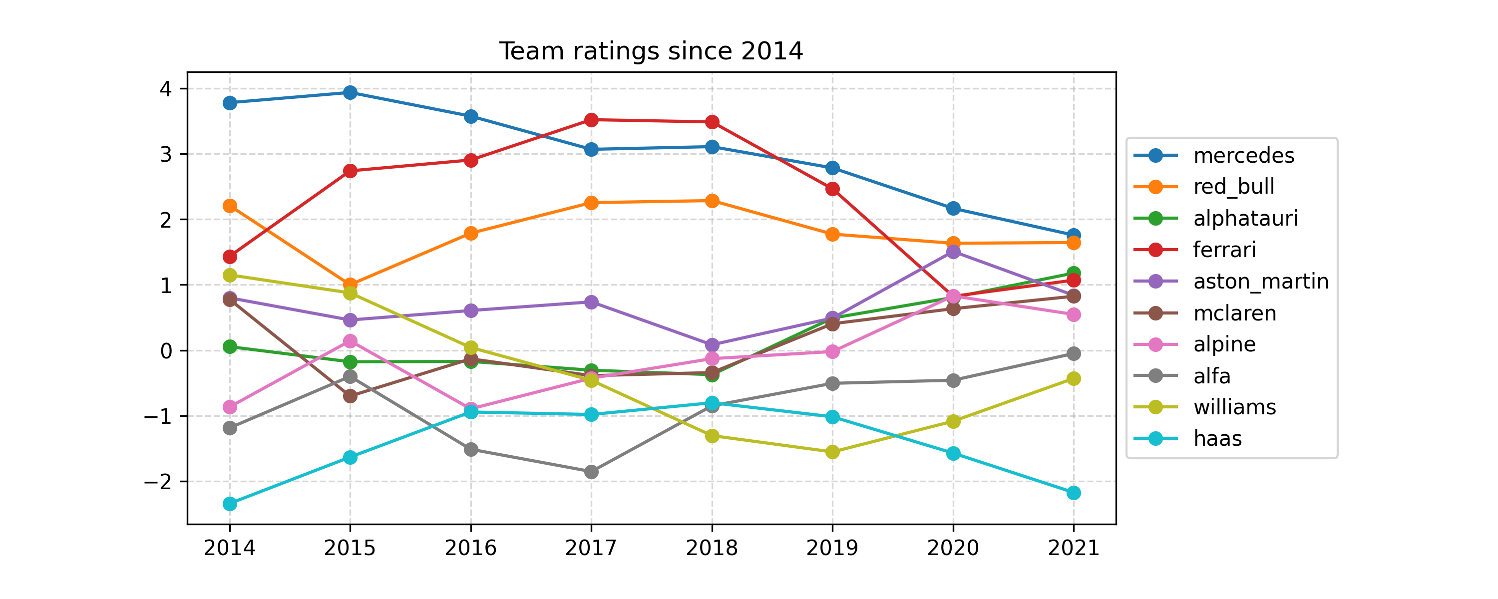
To interpret these values, remember the first equation in this post. For example, we can ask: what’s the probability, for an equally-skilled driver, that a Mercedes car will finish ahead of a Red Bull in 2014? We see that Mercedes had a rating of about 4, and Red Bull about 2. So, roughly:
\[p(\text{Mercedes ahead of Red Bull in 2014}) = \frac{\exp (4)}{\exp (4) + \exp (2)} \approx 88\%.\]That’s a pretty clear advantage, and Mercedes were very dominant in 2014, so that’s no surprise. Since then, Ferrari mounted a challenge, and the model actually rated their car slightly ahead of Mercedes’ in 2017 and 2018, which is interesting (and probably controversial). This year, Red Bull is rated as very close to Mercedes, and Ferrari have stopped a steep decline starting in 2018. There’s lots more that I could talk about here, but I’ll move on for now.
Driver ratings
Here are the mean inferred driver ratings over time. To show a manageable amount of drivers, I keep only those who were racing in 2016 and are still racing today:
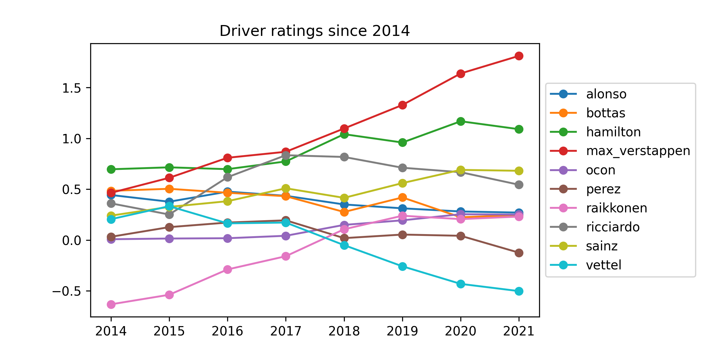
The first thing to notice is that the scale of these effects is quite a bit smaller than the car effects. That suggests that the car matters more than the driver. At the same time, these effects are by no means negligible, with almost two points separating Max Verstappen and Sebastian Vettel in the current ratings. I should note that Vettel, despite his poor performance here, is not the lowest rated current driver: Latifi, Tsunoda, Mazepin and Kubica are all behind him at the moment. Still, Raikkonen in 2014-2017 and Vettel since 2018 do not look great here.
Verstappen looks terrific here, and Hamilton has been consistently strong also. Here is the full current list of ratings:
max_verstappen     1.811
hamilton           1.090
norris             0.790
sainz              0.681
ricciardo          0.544
leclerc            0.495
russell            0.275
alonso             0.270
ocon               0.250
bottas             0.245
raikkonen          0.231
gasly              0.182
mick_schumacher   -0.081
perez             -0.124
giovinazzi        -0.141
stroll            -0.284
vettel            -0.502
latifi            -0.553
mazepin           -0.707
tsunoda           -0.976
kubica            -1.161
So you can see that according to this model, Verstappen is currently the highest-rated driver, followed by Hamilton. Norris, Sainz, Ricciardo and Leclerc are also rated highly; Latifi, Mazepin, Tsunoda and Kubica have the lowest ratings. Verstappen’s rating is really quite high: using the same logic as before, we can work out that his probability of beating Hamilton in the same car in a single race would be
\[p(\text{Verstappen beats Hamilton with same car}) = \frac{\exp (1.8)}{\exp (1.8) + \exp (1.1)} \approx 66.8\%.\]His edge over other drivers is, of course, even bigger. For example, against Mazepin:
\[p(\text{Verstappen beats Mazepin with same car}) = \frac{\exp (1.8)}{\exp (1.8) + \exp (-0.7)} \approx 92.4\%.\]But that probably isn’t very surprising to anyone!
It’s important to note a caveat here: Verstappen might look exceptional not because he’s so great, but because his team mates have underperformed. This model isn’t magic: the strongest signal for Verstappen’s skill comes from how well his team mates perform. It’s no secret that Red Bull has struggled to find a good second driver, and Gasly and Albon may not have been given enough time by Red Bull to adjust to their tricky car. Perez’s recent improvement has been credited in part to a better car setup, so that adds some weight to this idea.
DNFs
All the results above are conditional on the drivers actually finishing the race. What about the probability of them not finishing?
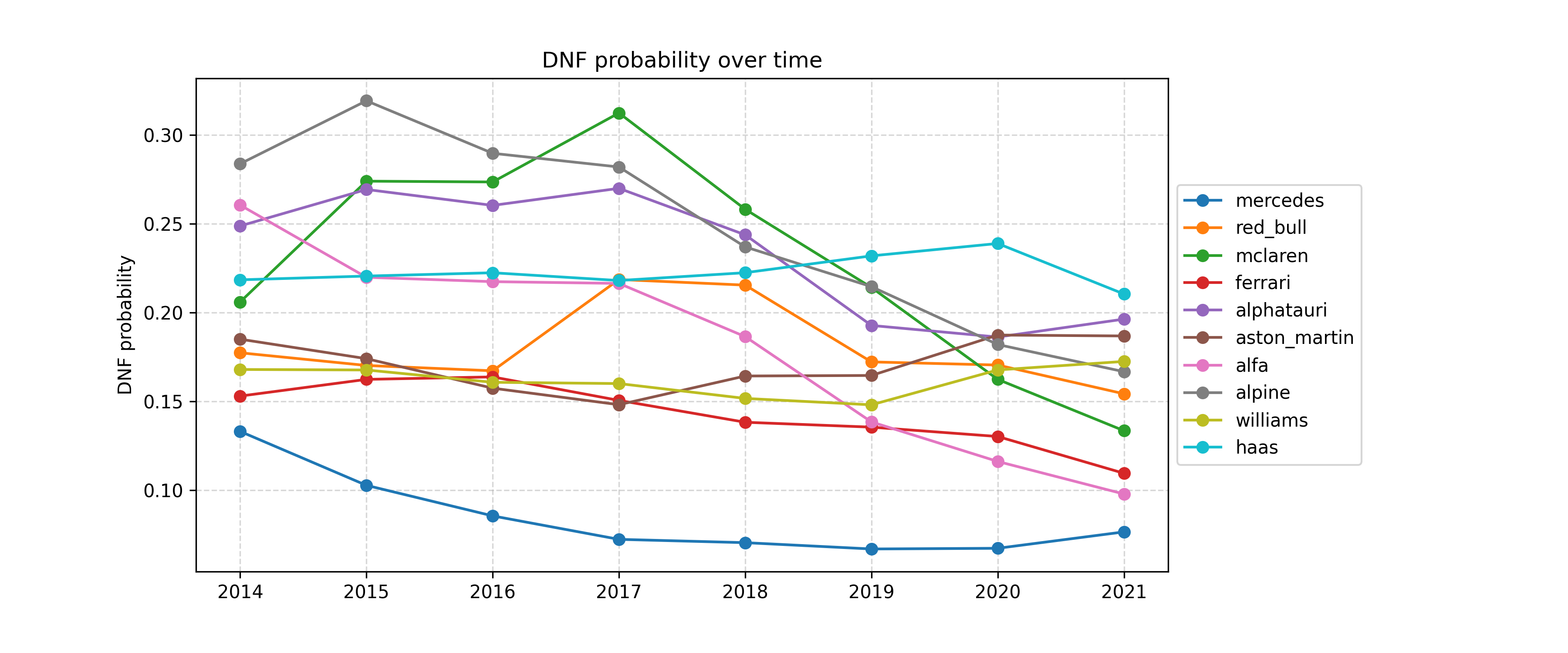
This is the probability of a DNF based only on the team. Look at how reliably Mercedes has been able to finish! That’s pretty astonishing. It seems that their ability to avoid DNFs is remarkable and is likely to play a role in their huge success.
What about the drivers? Here’s the current list of their effect (note that they’re on the logit scale; divide by 4 roughly to get the change in DNF probability when they are driving):
alonso             0.084
leclerc            0.069
stroll             0.034
max_verstappen     0.013
tsunoda            0.013
russell            0.012
raikkonen          0.004
latifi            -0.002
ocon              -0.003
mazepin           -0.005
bottas            -0.010
ricciardo         -0.016
norris            -0.020
sainz             -0.022
kubica            -0.023
giovinazzi        -0.024
gasly             -0.027
mick_schumacher   -0.038
vettel            -0.043
hamilton          -0.075
perez             -0.126
These effects are all quite small, but they suggest that drivers like Leclerc and Alonso take the most risk, and Perez and Hamilton are least likely to crash out.
Who wins this year?
Putting all this together, what does this mean for points? We saw that the Red Bull and Mercedes cars are closely matched, and Verstappen is estimated to be the best driver, but also that the Mercedes is apparently more reliable. To be precise, it turns out that Hamilton has roughly 7.2% probability of DNFing, while Verstappen’s probability is about 17.8%. So how do these things balance out? We can simulate races and compute the points won for each. Once we do that, we get the following expected points per race:
max_verstappen     14.54
hamilton           14.18
bottas              9.84
sainz               7.74
leclerc             7.11
norris              6.95
perez               6.47
ricciardo           6.22
gasly               5.23
alonso              3.87
ocon                3.57
stroll              2.87
raikkonen           2.37
vettel              2.34
tsunoda             2.20
giovinazzi          1.83
russell             1.72
latifi              0.81
kubica              0.77
mick_schumacher     0.23
mazepin             0.14
Look at how closely Verstappen and Hamilton are matched! So their close title contest is no surprise according to the model. Bottas in third makes sense, but I am quite surprised to see Perez so low. That’s something I want to investigate, but I suspect it’s because he had some poor results before the most recent races, finishing 9th in Russia, 8th in Zaandvort, and 19th in Belgium, just to name a few. It feels like he’s got a better feel for the car now, but the model does not account for within-season changes in skill, so that might be something else to look at.
We can also simulate races to see how likely it is that Hamilton can make up the 14 point deficit currently separating him from Verstappen. It turns out that this probability is currently 24% under the model, so Verstappen is the favourite, but a Hamilton comeback wouldn’t be out of the question.
Things I’d like to improve
This is just a start; there are lots of things to try in the future. Among them:
- Track effects: Some tracks favour some cars, and it might be interesting to try to infer that.
- Data on within-race issues: If I had data on crashes and mechanical issues during the race, that could be used to refine the model.
- Using more data: With some modifications to account for changes in eras, it could be interesting to go further back in time.
- More evaluation: I haven’t really tried to predict a hold-out set here, so I don’t know how well this model does at prediction
- A “first year in car” effect: I wonder if it the first year in a car is particularly tricky – just see how Ricciardo and Perez seem to have had a tough time in their first years in the McLaren and Red Bull cars, respectively.
Summary
I hope you enjoyed this brief look at my first Formula 1 model. I’m interested to hear feedback from people who are long-time F1 fans. Does something look terribly off? Is anything clearly missing? Send me an email, or reply to the Tweet!
Appendix: Code
If you’re interested in fitting this model yourself, take a look at this repository. I haven’t had time to tidy the Jupyter notebook there a great deal, but I hope the code is still helpful to get started.