This post is a short note on how to add random effects to GPs. It took me some time to understand how to do this, and I’m hoping that this short writeup could help some others who are curious about how it can be done.

A motivating example

To motivate this, let’s consider the problem of estimating how the average rally length by surface changed over time in men’s tennis. A source we can use for this is the Match Charting Project, whose earliest matches are from the early 70s. Here’s what the data look like:

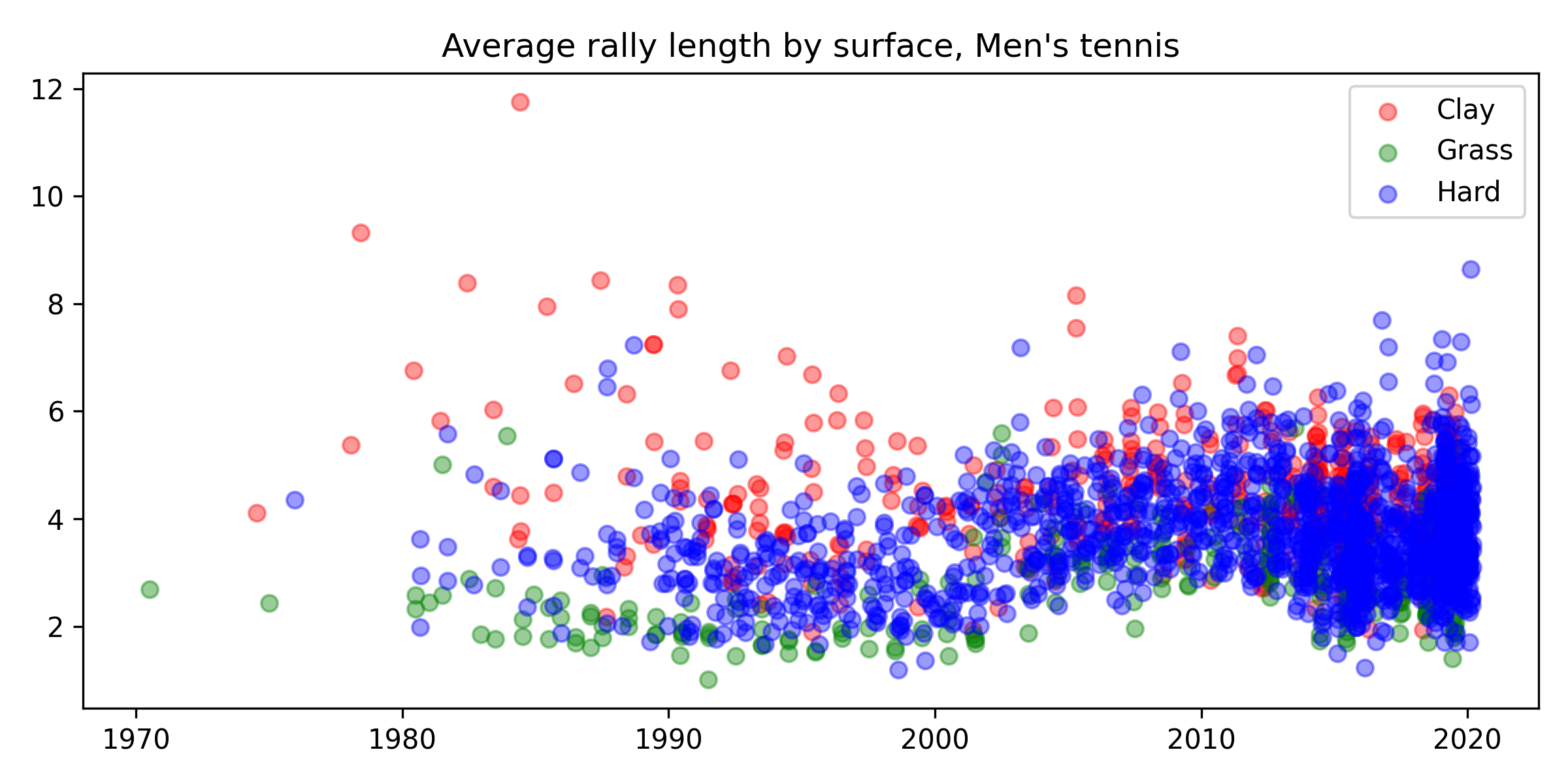
Each point here is the average rally length in a match, and each point is coloured by the surface the match was played on. It appears that clay court rallies tend to be longest, followed by hard courts, and finally grass courts. It would be nice to smooth the trends over time with a GP.

How can we fit this data with a GP? We can approximate the likelihood as Gaussian, and the dataset isn’t too big (2,513 matches), so we don’t need to resort to any fancy approximations. That’s all good, but which kernel to pick?

The kernel on time is easily chosen, I think. We’ll want one of the usual suspects – a Matern kernel, or a radial basis function (RBF) kernel. The first challenge is how to incorporate surface. Here, David Duvenaud’s excellent kernel cookbook can help us out (section: “How to use categorical variables in a Gaussian Process regression”). We encode the categorical variables as one-of-$k$ (sometimes also called “one-hot” encoding) and put a product of RBF kernels on them. Then we multiply this kernel with the time kernel to have high covariance only when points are close in time and on the same surface.

Here’s the result we get with those kernels:

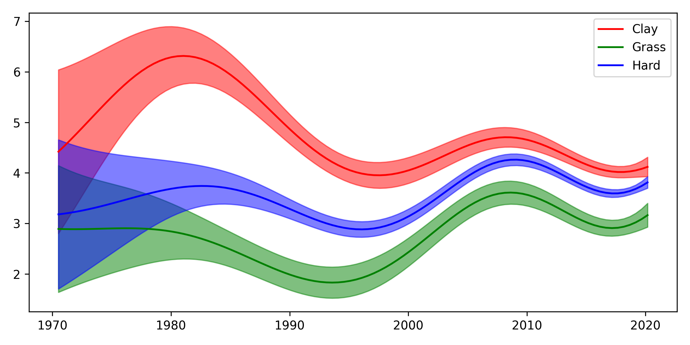
This is quite nice: it matches general domain knowledge – surfaces became more homogeneous since 1990, for example.

But we also have player effects. Some players will tend to play longer rallies than others. If many of the charted matches in the 80s on clay, for example, involve the same player who plays extremely long rallies (looking at you Mats Wilander), we might be overestimating the actual mean rally length in that period.

How do we incorporate player effects? We could model the mean rally length in match $i$ as follows:

\[f_i = \eta_i + \gamma_{p_1(i)} + \gamma{_{p_2(i)}},\]

where $\eta_i$ is the effect of surface and time (handled by the kernel we just discussed), and we have added $\gamma_{p_1(i)}$ and $\gamma_{p2(i)}$, the effect of player 1 and 2 on rally length. To make this a random effects model, we’ll also assume:

\[\gamma_j \stackrel{iid}{\sim} \mathcal{N}(0, \sigma^2).\]

Note that in general we could assume non-zero mean, but here we are modelling offsets from the time and surface mean, so it makes sense for them to have a prior of zero.

That’s all very well, but this isn’t a kernel function. How do we find an equivalent kernel?

The random effects kernel

The first trick, which is not actually necessary but simplifies our life a bit, is to rewrite the expression for $f_i$ as follows:

\[f_i = \eta_i + z_i^{T}\gamma.\]

Here, $\gamma$ is the vector of all random effects, and $z_i$ is a vector with ones at $p_1(i)$ and $p_2(i)$ and zeros everywhere else. With a little bit of thought it should be easy to convince yourself that this is equivalent to the previous version.

Now we pull the second trick, which is often useful in deriving kernel functions. We consider a second arbitrary function value, at point $j$:

\[f_j = \eta_j + z_j^T \gamma.\]

Then we compute the covariance between $f_i$ and $f_j$:

\[cov(f_i, f_j) = cov(\eta_i + z_i^T \gamma, \eta_j + z_j^T \gamma).\]

Now we just need to use some properties of the covariance. First, note that we can split things up:

\[cov(\eta_i + z_i^T \gamma, \eta_j + z_j^T \gamma) = cov(\eta_i, \eta_j) + cov(\eta_i, z_j^T \gamma) + cov(z_i^T \gamma, \eta_j) + cov(z_i^T \gamma, z_j^T \gamma).\]

Things now simplify quite a lot. The first term is just the kernel function we’ve discussed for time + surface. The second and third terms are zero, since we assume that $\eta_i$ and $\gamma$ are independent in the prior. That leaves the final term:

\[cov(z_i^T \gamma, z_j^T \gamma)= z_i^T cov(\gamma, \gamma) z_j,\]

where I’ve used a standard result for vector covariances multiplied by (constant) matrices. We had that

\[\gamma_j \stackrel{iid}{\sim} \mathcal{N}(0, \sigma^2),\]

so

\[\gamma \sim \mathcal{N}(0, \sigma^2 I),\]

and

\[cov(z_i^T \gamma, z_j^T \gamma) = \sigma^2 z_i^T z_j.\]

This completes the “random effects kernel”, which actually is nothing but a linear kernel! The kernel function is:

\[k_{raneff}(z_i, z_j) = \sigma^2 z_i^T z_j.\]

If $Z_1$ and $Z_2$ are matrices of shape $N \times M$ and $D \times M$, we can compute all covariances at once as follows:

\[k_{raneff}(Z_1, Z_2) = \sigma^2 Z_1Z_2^T.\]

The result

The full kernel function is:

\[k_{full} = k_{ts} + k_{raneff},\]

the first being the product of RBF kernels on time and surface, and the second being the random effects kernel.

The first thing we can do is predict only $k_{ts}$, the time and surface component. It looks like this:

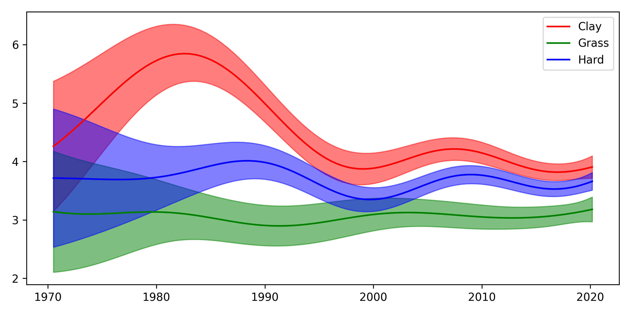
The plot looks similar to the previous one, but not the same. To be quite honest, I’m not sure I like it better! For one, I think most viewers of tennis would agree that rally lengths on grass have got a bit longer over time, but in this new plot, we don’t really see much of that. Perhaps we need an even more complex model, like surface-specific random effects? I’m not entirely sure at this point.

We can also take a look at the estimated random effects for the players. Of players with at least 10 matches played, here are the fifteen who are estimated to extend rallies the most:

	mean	sd
Gilles Simon	1.38	0.13
Mats Wilander	1.19	0.16
Guillermo Coria	1.17	0.18
Alex De Minaur	0.93	0.13
Roberto Bautista Agut	0.86	0.11
Andy Murray	0.8	0.06
Thomas Muster	0.73	0.16
David Ferrer	0.69	0.09
Novak Djokovic	0.69	0.05
Alex Corretja	0.66	0.19
Jimmy Connors	0.66	0.17
Lleyton Hewitt	0.66	0.08
Diego Sebastian Schwartzman	0.65	0.17
Guido Pella	0.64	0.17
Marton Fucsovics	0.57	0.16

As you’d expect, Mats Wilander is high up here (just look at this rally – not actually the longest ever, but still), and I think the others seem mostly reasonable too. Gilles Simon tops the list: rallies against him are expected to be 1.38 shots longer than usual.

We can also look at the fifteen who are estimated to shorten rallies the most:

	mean	sd
Ivo Karlovic	-1.46	0.12
John Mcenroe	-1.43	0.16
Richard Krajicek	-1.02	0.19
John Isner	-0.94	0.1
Dustin Brown	-0.93	0.16
Stefan Edberg	-0.89	0.09
Reilly Opelka	-0.86	0.19
Milos Raonic	-0.82	0.1
Pete Sampras	-0.77	0.09
Patrick Rafter	-0.75	0.14
Michael Stich	-0.72	0.17
Alexander Bublik	-0.71	0.17
Marco Cecchinato	-0.62	0.18
Boris Becker	-0.6	0.12
Denis Shapovalov	-0.59	0.11

This seems to be a mix of serve-volleyers and big servers, which also seems reasonable. Don’t expect long rallies if you’re watching a Karlovic - Opelka match, for example.

Overall, I hope you found this blog post interesting. Personally, I think adding random effects to GPs can be a reasonable thing to do a lot of the time, and I’m likely to use the “random effects kernel” a fair bit in the future.

UPDATE (28th March 2021): The code I used to fit the GP in this blog post is now available here.