Last week, I wrote about random effects in GPs, motivated by smoothing rally lengths over time in tennis. I’d thought this would be quite a niche topic, but to my surprise, it got a fair bit of interest. I was humbled to receive comments from some of my favourite GP researchers. Neil Lawrence, one of these people, made the following suggestion:

Nice work Martin. My instinct would have been to do it in log space … Use the same additive covariance, but random effect is now a multiplier … which also feels like it makes more sense for rally length (both for surface and player) That might give more interpretability.

(see here for the original tweet)

I thought this was a great idea. As I replied to Neil, in addition to potentially improving the interpretation, this would also have the effect of avoiding negative rally length predictions, which of course don’t make sense. So I gave it a go – here’s what I found.

The model in log space

The way I went about this was to first transform the data, $y$, to $\log y$. Modelling $\log y$ with a Gaussian implies that we think the outcome is log-normally distributed. As Neil suggested, we can use the same model as before, which was:

\[f_i = \eta_i + \gamma_{p_1(i)} + \gamma_{p_2(i)}.\]

Here, $\eta_i$ is the smooth trend from surface and time, and the $\gamma$ are offsets (if you’d like to know more, please check out the previous post). The difference is that since we are now modelling the log of the rally length, the additive effects here are in fact multiplicative. To be concrete, we are modelling:

\[\log y_i = \eta_i + \gamma_{p_1(i)} + \gamma_{p_2(i)} + \epsilon_i,\]

so

\[y_i = \exp(\eta_i + \gamma_{p_1(i)} + \gamma_{p_2(i)} + \epsilon_i) = \exp(\eta_i) \exp(\gamma_{p_1(i)})\exp(\gamma_{p_2(i)}) \exp(\epsilon_i),\]

where $\epsilon_i$ is iid Gaussian noise, and I multiplied things out to be extra-clear that these are now multiplicative effects. Overall, this means that if e.g. $\gamma_{p_1(i)}$ is 0.5, $\exp(0.5) \approx 1.65$, so the effect of player $p_1(i)$ would be to extend rallies by a multiple of 1.65.

The new result

Once we’ve fit the GP to $\log y$, we can put the predictions back on the non-log scale by exponentiating the function values. To help with this, we can make use of some properties of the log-normal distribution. Calling $f_i$’s mean $\mu_i$ and its variance $\sigma^2_i$, the mean is:

\[\mathbb{E}[\exp(f_i)] = \exp\left(\mu_i + \frac{\sigma_i^2}{2}\right),\]

and the variance is:

\[\textrm{Var}(\exp(f_i)) = (\exp(\sigma_i^2) - 1)\exp(2 \mu_i + \sigma_i^2).\]

This will allow us to make the same plot as previously. First though, let’s remember what that previous plot looked like:

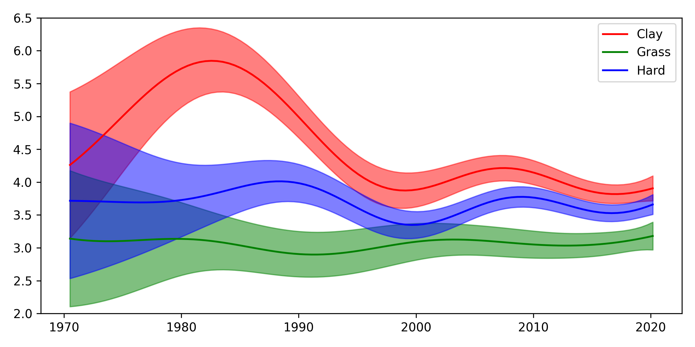
Now, here’s the new one:

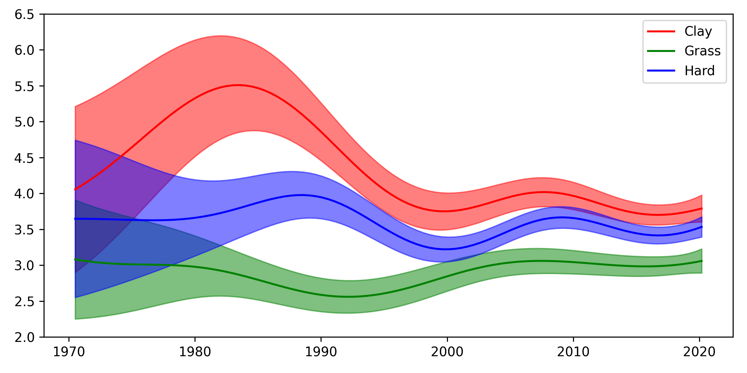
Superficially, the two are very similar, but if you look closely, there are some small differences. One slight difference is that the new plot shows a bit more of an increase in rally lengths on grass since the 1990s, which is more in line with what I would have expected (though more on this in a moment). The error bars are also somewhat different. It might be interesting to investigate model fit with some kind of model selection technique to see whether there is a way to choose between these two models in a quantitative way. I’m interested to hear suggestions if you have them!

New player effects

We can also take a look at the new multiplicative player effects. Here are the players estimated to extend rallies the most:

	mean	exp(mean)	sd
Gilles Simon	0.31	1.36	0.03
Mats Wilander	0.26	1.3	0.04
Guillermo Coria	0.26	1.29	0.05
Roberto Bautista Agut	0.23	1.26	0.03
Alex De Minaur	0.22	1.25	0.03
Andy Murray	0.2	1.22	0.02
Lleyton Hewitt	0.19	1.21	0.02
Diego Sebastian Schwartzman	0.19	1.2	0.04
Jimmy Connors	0.18	1.2	0.04
Alex Corretja	0.18	1.2	0.05
Thomas Muster	0.18	1.19	0.04
Novak Djokovic	0.18	1.19	0.01
David Ferrer	0.17	1.19	0.02
Marton Fucsovics	0.17	1.18	0.04
Guido Pella	0.16	1.18	0.04

This suggests that rallies against Gilles Simon are on average around 36% shots longer than usual, for example. It also means that a hypothetical match between Wilander and Simon on clay in the eighties would have an expected average rally length of about $1.36 \times 1.3 \times 5.5 \approx 9.7$ shots – not bad! That would put it not too far off from the highest recorded average rally length, which was 11.8, between Mats Wilander and Ivan Lendl at the French Open in 1984. Alas, we will never witness this epic slugfest.

And here are the fifteen who are estimated to shorten rallies the most:

	mean	exp(mean)	sd
Ivo Karlovic	-0.51	0.6	0.03
John Mcenroe	-0.37	0.69	0.04
Richard Krajicek	-0.35	0.7	0.05
Dustin Brown	-0.31	0.73	0.04
John Isner	-0.3	0.74	0.03
Reilly Opelka	-0.29	0.75	0.05
Patrick Rafter	-0.27	0.76	0.04
Stefan Edberg	-0.26	0.77	0.02
Pete Sampras	-0.25	0.78	0.02
Milos Raonic	-0.24	0.79	0.02
Alexander Bublik	-0.22	0.8	0.04
Goran Ivanisevic	-0.21	0.81	0.04
Michael Stich	-0.2	0.82	0.04
Boris Becker	-0.19	0.83	0.03
Todd Martin	-0.18	0.84	0.05

This suggests, for example, that rallies against Karlovic are only expected to be about 60% of their usual length.

Both lists are similar to the previous ones. The list of players extending rallies the most contains the same names, they’re just shuffled a little bit. In the second list of players who shorten rallies the most, Marco Cecchinato and Denis Shapovalov no longer make the top 15; instead, we’ve gained Goran Ivanisevic and Todd Martin, which I think makes sense.

Finally, I wanted to mention a comment made by another GP researcher whose work I’m a fan of, James Hensman:

What a neat post on random effects modelling with kernels. Also: tennis!

Seems that when we account for player-wise effects, grass rallies have not got longer. Maybe this makes sense: it’s the players making the matches longer, the surface itself remains the same.

(original tweet)

I think James makes an interesting point, particularly when you look at the players who shorten rallies the most. A lot of those players are famous for their success on grass: eight of them (McEnroe, Krajicek, Rafter, Edberg, Sampras, Ivanisevic, Stich, Becker) won Wimbledon at least once. In the past, it appears that Wimbledon rewarded players with these styles. These days, for whatever reason – perhaps better racket or stringing technology – baseliners can do very well there, and this might explain much of the increasing trend in rally lengths.

In any case, I hope you’ve enjoyed this second look at rally lengths. I agree with Neil that the version in log space seems more compelling. It definitely seems worth asking yourself “would modelling $\log y$ be better?” whenever you’re modelling positive data, and it’s something I’ll do more often in the future.