Last week, I wrote about JAX ADVI, a little library I put together for fast black-box variational inference using JAX. As I mention in that post, the version implemented in the package uses an improved version of ADVI, as suggested by Giordano, Broderick and Jordan. The main topic of their paper is actually something else, though: they justify and evaluate a method called “linear response variational Bayes” (LRVB). It promises to get accurate estimates of posterior variances and covariances from ADVI and other variational inference methods. In this post, I’ll talk a bit about this approach and my experience of implementing it in JAX.

The paper provides proofs that I haven’t yet worked through in detail, so I won’t talk about the paper’s derivations in this post. Instead, I want to highlight a key result that’s useful for ADVI. That result is the following posterior covariance estimate:

\(\textrm{Cov}_{q_0}^{LR}(\theta) = \begin{bmatrix} I_K & 0 \\ 0 & 0 \end{bmatrix} \mathbf{H}_{\eta \eta}^{-1} \begin{bmatrix} I_K & 0 \\ 0 & 0 \end{bmatrix}\).

Here, $\mathbf{H}_{\eta \eta}^{-1}$ is the inverse of the Hessian of the variational objective, evaluated at the optimum, and $\eta$ is the vector of variational parameters. The first half of $\eta$ is made up of the variational means, and the second is made up of the (log) standard deviations. The dimension of $\eta$ is $K$, and $I_K$ is the identity matrix of size $K \times K$.

The equation says that to get the LRVB estimate of the posterior covariance, we have to compute the Hessian of the objective at the optimum, invert it, and pick out the top left $K \times K$ corner. If computing and inverting the Hessian reminds you of the Laplace approximation, that’s no accident: Giordano et al. suggest that the Laplace approximation can be thought of as a special case of their method.

Does it work? The short answer is yes, at least in the few cases I’ve tried so far. Here’s code to make some fake data for a logistic regression:

import numpy as np
from jax.nn import sigmoid

N = 1000
K = 10

np.random.seed(2)

X = np.random.randn(N, K)
beta_true = np.random.randn(K)
gamma_true = np.random.normal()

logit_true = X @ beta_true + gamma_true

y = np.random.uniform(size=N) < sigmoid(logit_true)

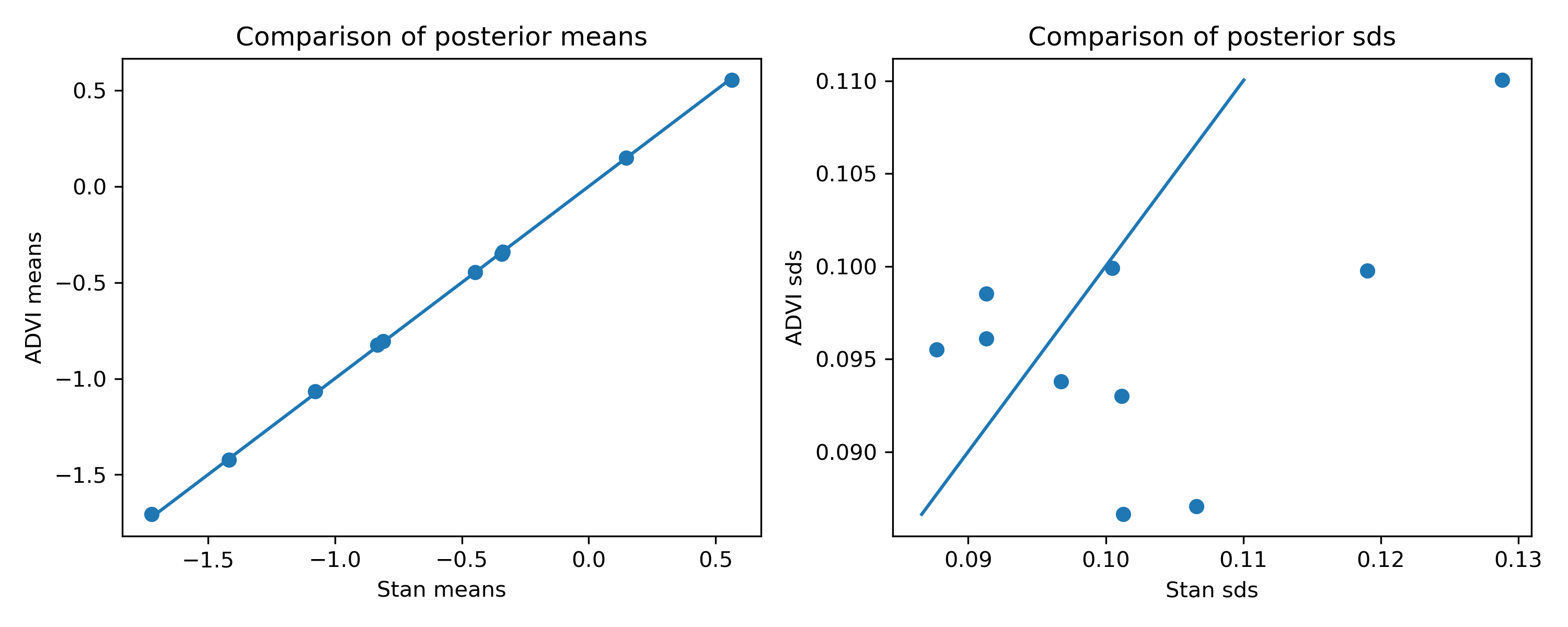
In the previous blog post, I plotted the inference results from Stan’s MCMC sampler against those from mean-field ADVI:

As you’d expect with a mean-field objective, the means are good, but the standard deviations are off.

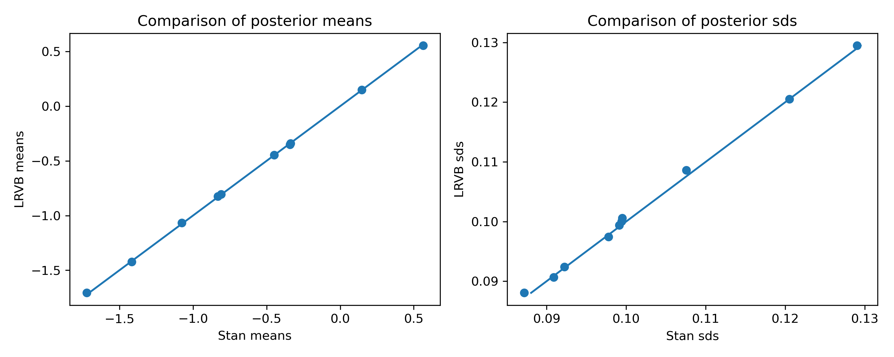
Here’s what we get with LRVB:

Nice! The standard deviations are now almost exactly the same as in Stan.

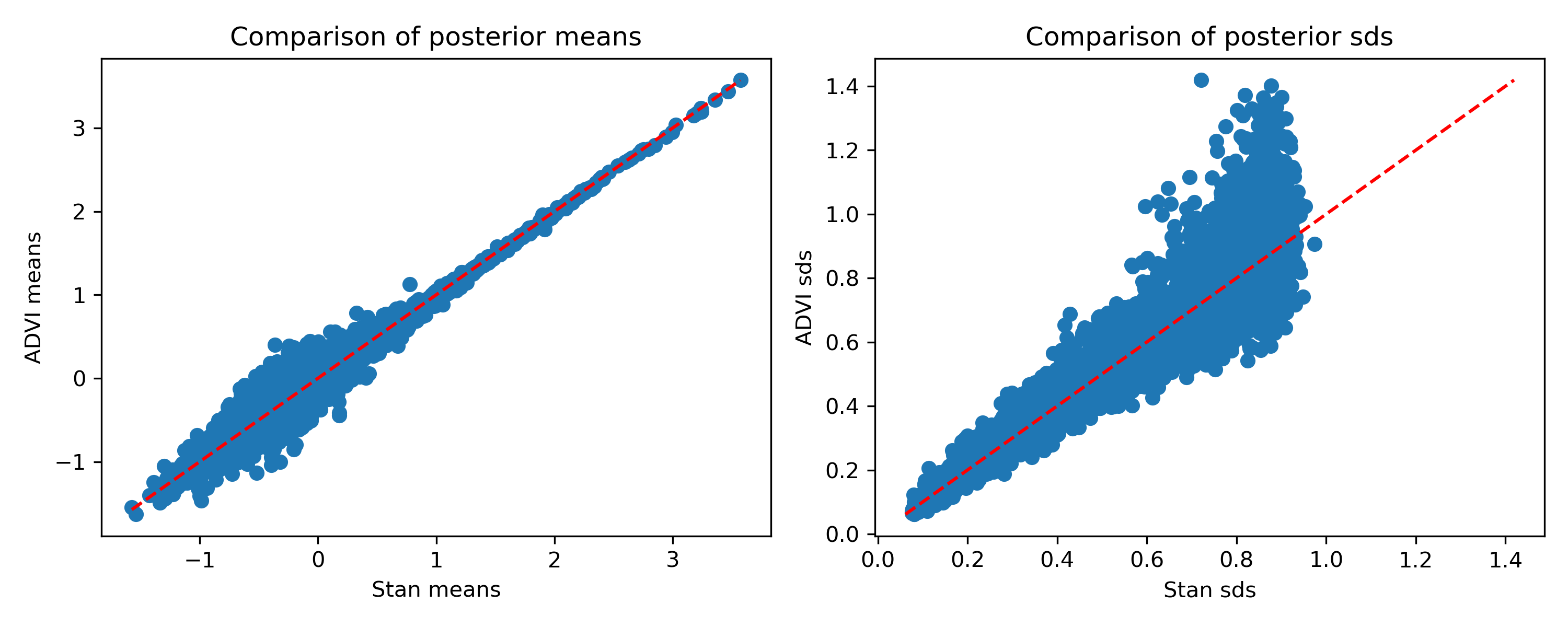
What about a more complex example? Here’s a hierarchical Bradley-Terry model (details for it are in the previous post). It consists of 158,394 matches between 4,763 competitors. For the player skill posteriors, ADVI gives:

Again, the means are quite good, but the standard deviations are off. Note that the means don’t look as good here. I’ve noticed that they get better as we increase the number of samples in the Monte Carlo estimate for the variational objective. Here, I’m using just 25. With 25, LRVB takes about five minutes; with 100 it takes about 13 minutes. So you can choose a time/accuracy tradeoff depending on the level of accuracy required. For reference, Stan took about 100 minutes on this example. Giordano et al. have a clever way to choose the number of MC samples which I have yet to try.

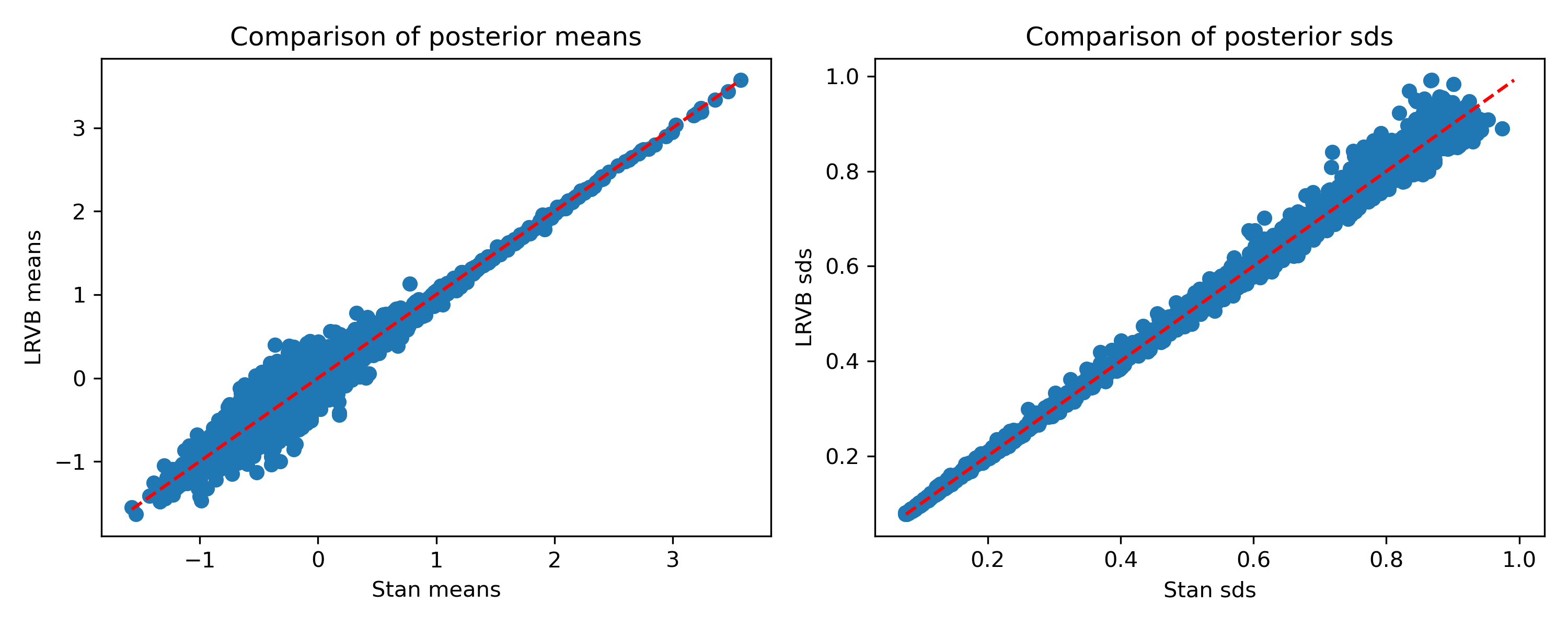
Here’s how the result changes with LRVB:

Much better, once again!

You might ask why you’d use this over the Laplace approximation. I think the key benefit of this approach is that it can handle hierarchical models. It’s well-known that the MAP estimate in hierarchical models often sets the group variance to zero, which results in a singular Hessian. You can get around that by doing a nested Laplace approximation, which is what INLA does, but it complicates things because you now have to do nested optimisations, whereas LRVB only requires a single one. I think it would be very interesting to compare INLA and LRVB in more depth.

Caveats

The main caveat with LRVB is that it doesn’t scale as well as mean-field VB. As I’ll talk about in the addendum (if you’re interested in that sort of thing), the implementation in JAX ADVI basically works by computing lots of matrix-vector products with the Hessian. The Hessian’s shape will be $2K \times 2K$, where $K$ is the number of parameters. For the example above, with about 4000 parameters and 160,000 data points, this means there will be lots of matrix-vector multiplications with a $8000 \times 8000$ matrix. That still seems to work pretty quickly in JAX as mentioned, but if your problem has an order of magnitude more parameters, I would expect things to slow down a lot. Basically, the current implementation’s complexity is likely to be at least $\mathcal{O}(K^3)$, so I’d expect it to work best when there are maybe at most 10,000 parameters.

That said, Giordano et al. do have a trick: they partition the parameters into global parameters, like group variances in a hierarchical model, and local parameters, like the player skills in the tennis example. It turns out that the Hessian will end up being sparse because the cross terms between local parameters will be zero. In the interest of having a completely black-box implementation, I haven’t tried this yet, but it would be interesting to try this in the future.

Another caveat is that even if LRVB gets the variances and covariances right (and I haven’t really checked the latter yet), it still only matches the first two moments, so if the posterior is highly skewed or multi-modal, it won’t necessarily be a faithful approximation.

Summary

I think LRVB is really cool: it gives you an intermediate option between mean field VB, which gets the means right and is super-quick, and HMC, which should be almost exact but can be slow. If you’d like to try it for yourself, you can. The logistic regression example is here and the tennis example is here. Note that the LRVB implementation is still experimental and I might change the API a little!

Addendum: Implementation in JAX

Implementing LRVB in JAX was almost shockingly easy. I’d expected it to take me some time to get going but amazingly, it worked almost instantly. That’s largely because the important operations are already implemented in JAX.

The idea I used to implement LRVB in JAX is suggested in Giordano et al.. Basically, looking at the key equation:

\(\textrm{Cov}_{q_0}^{LR}(\theta) = \begin{bmatrix} I_K & 0 \\ 0 & 0 \end{bmatrix} \mathbf{H}_{\eta \eta}^{-1} \begin{bmatrix} I_K & 0 \\ 0 & 0 \end{bmatrix}\),

we see that we can first compute

using a solve operation. I’ve dropped the columns of zeros on the right since they’ll just stay zero. This will produce a matrix of size $K \times 2K$, and we can then pick out the top $K \times K$ block to get our desired covariance estimate.

Inverting the Hessian is expensive. Actually, even computing it explicitly could be too costly: as mentioned, it’s $2K \times 2K$, and $K$ can be large. However, we can use something called the conjugate gradients algorithm to avoid ever forming it explicitly. Basically, given a linear system $Ax = b$, it solves for $x$ using only matrix-vector products between $A$ and a vector. In our case, we can use conjugate gradients $K$ times, one for each column of \(\begin{bmatrix} I_K \\ 0 \end{bmatrix}\), using only matrix multiplications between vectors and the Hessian.

Why is that good? The cool thing is that JAX can efficiently compute exactly such products without actually forming the Hessian. The operation is called the Hessian vector product, or hvp for short. Even better, JAX can not only compute these efficiently, it also supports the conjugate gradients algorithm, so I didn’t have to write it myself. One little trick I’ve added is to use the mean field variance estimates as a preconditioner, which I don’t remember from the Giordano et al. paper but they probably thought of that too. In any case, the final implementation is basically just a few lines long and you can check it out here if you like.