If you have a great memory, you might remember that about five years ago, I posted about deterministic ADVI in JAX, or DADVI for short. That kicked off some work with the wonderful Ryan Giordano and Tamara Broderick, and we worked on a paper together that investigated DADVI in depth. I feel very grateful to have worked with such brilliant coauthors.

Now, I’m excited to say that a first version of DADVI is part of pymc-extras, which means that it’s easy to fit PyMC models with DADVI. Well, not all of DADVI yet – it doesn’t yet include its linear response component (more on that in a bit) – but it already removes the convergence worries, so I thought I’d write a short post about this.

What’s Black Box Variational Inference?

One of the great things about Bayesian statistics is that you have a lot of freedom. You specify your model, and then software like PyMC and Stan gives you samples from the posterior distribution using Markov Chain Monte Carlo (MCMC). However, if you’ve tried to fit models with a lot of parameters or a lot of data, you might have noticed that MCMC can take quite a while to run – sometimes, too long to be practical.

In these cases, if you’re willing to compromise a bit, you can try an approximate method. One such method is mean-field variational inference with Gaussians. This method tries to approximate the posterior with one-dimensional Gaussian distributions, one for each parameter. By definition, this can’t capture any of the covariance information. And it often underestimates the variances, too. But, at least in many cases, it can give you good estimates of the posterior means, and it can be much faster than MCMC.

To get a feel for this, here’s what happens when you fit mean-field variational inference to a bivariate Gaussian distribution with mean zero, marginal variances of 1, and correlation coefficient equal to 0.8:

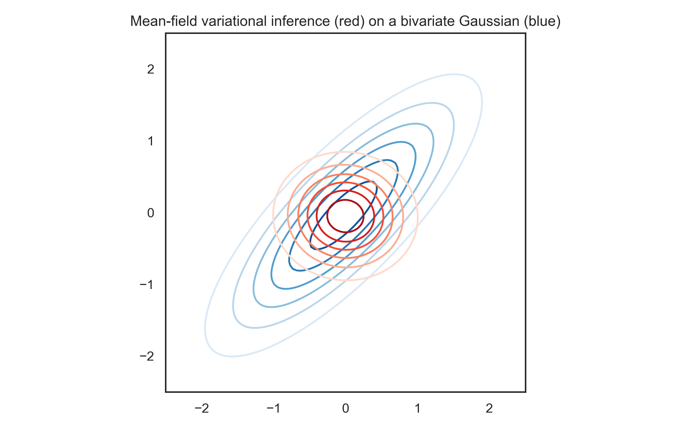
The bivariate normal is in blue, and the approximation in red. As you can see, it gets the means pretty much right, but it underestimates the variance and it completely misses the correlation. But getting the means right can already be pretty useful.

What’s wrong with the black box method in PyMC?

PyMC has supported a very general version of mean-field variational inference called ADVI (automatic differentiation variational inference) for some years now. So why do we need DADVI?

Well, it turns out that ADVI has some problems, and DADVI can help with some of them. Three stand out:

1. It’s not easy to tell when ADVI has converged
2. Like other variational inference methods, ADVI underestimates the posterior variances
3. Sometimes, especially in complex models, ADVI even fails to estimate the posterior means correctly.

DADVI fixes (1) and, with something called linear response theory, can help with (2). It doesn’t solve all the problems, though: when the variational objective fails to capture important parts of the posterior, it can still provide a bad approximation even to the means, so (3) can still be a concern. So it’s best to be a bit careful and not blindly trust what variational inference gives you.

The PyMC implementation of DADVI doesn’t include the linear response parts yet, so it’ll only fix the convergence issues, not the variances. But as you’ll see in a moment, I think that can already make life a bit easier.

Tennis example

Rather than just talking about it, I thought it might be fun to demonstrate how DADVI works on an actual example. I like tennis, so I used Jeff Sackmann’s Tennis ATP dataset to fit a model to estimate players’ serve and return skill. It’s the same model I fit here, but we have some more years of data since then, so it’ll be fun to see where the new players end up. Using all data available starting from 1990, the dataset contains about 96k matches between about 2k players, so it’s fairly big.

The model is a hierarchical linear regression, and it models the probability $p$ that a player wins a point on serve:

For example, if Federer had a serve skill of 0.5, and Nadal had a return skill of 0.3, and the intercept is 0.5, then his expected probability of winning a point on serve would be $\text{logit}^{-1}(0.7) \approx 67\%$. The inverse logit function makes sure that the result is always between 0 and 1.

The server and return skills are given hierarchical priors. I won’t go into more detail here, but I’ll put the full model as well as its code in PyMC at the end if you’re interested.

Once the model is defined, we can try different inference methods in PyMC. For example, we can fit ADVI as follows:

with m:
	advi_res = pm.fit().sample(draws=1000)

By default, this runs ADVI for 10000 iterations, which takes about 80 seconds on my laptop (an Apple MacBook Pro 13 inch from 2020 with an M1 chip). Pretty quick for almost 100k data points! But let’s see if it actually did a good job. We can fit PyMC’s default sampler like so:

with m:
	idata_nuts = pm.sample()

This takes about 10.5 minutes, so it’s definitely slower (though to be honest, it’s pretty impressive for MCMC given the size of the dataset). But it should do a good job at capturing the posterior distribution. Now we can compare the mean serve skill estimates from ADVI and MCMC:

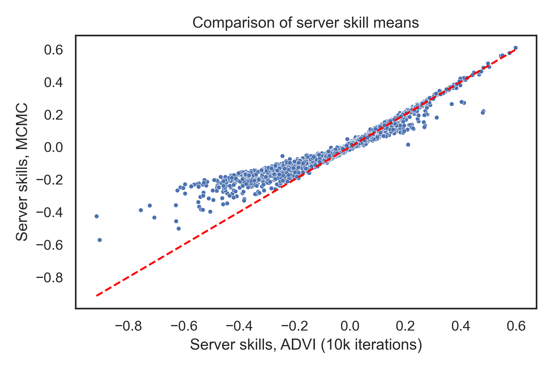
Here, each point on the scatter plot is a player’s serve skill, and the dashed red line indicates equality. If ADVI matched the MCMC means, all the points would lie on or near the dashed line. But while there’s definitely some correlation here, many points are pretty far off. Maybe it hasn’t converged? Let’s run it for longer – 100k iterations – and include its convergence criterion so it can stop early if it’s converged:

from pymc.variational.callbacks import CheckParametersConvergence
with m:
	advi_res_convergence_crit = pm.fit(
	n=100000, 
	callbacks=[CheckParametersConvergence()]).sample(draws=1000)

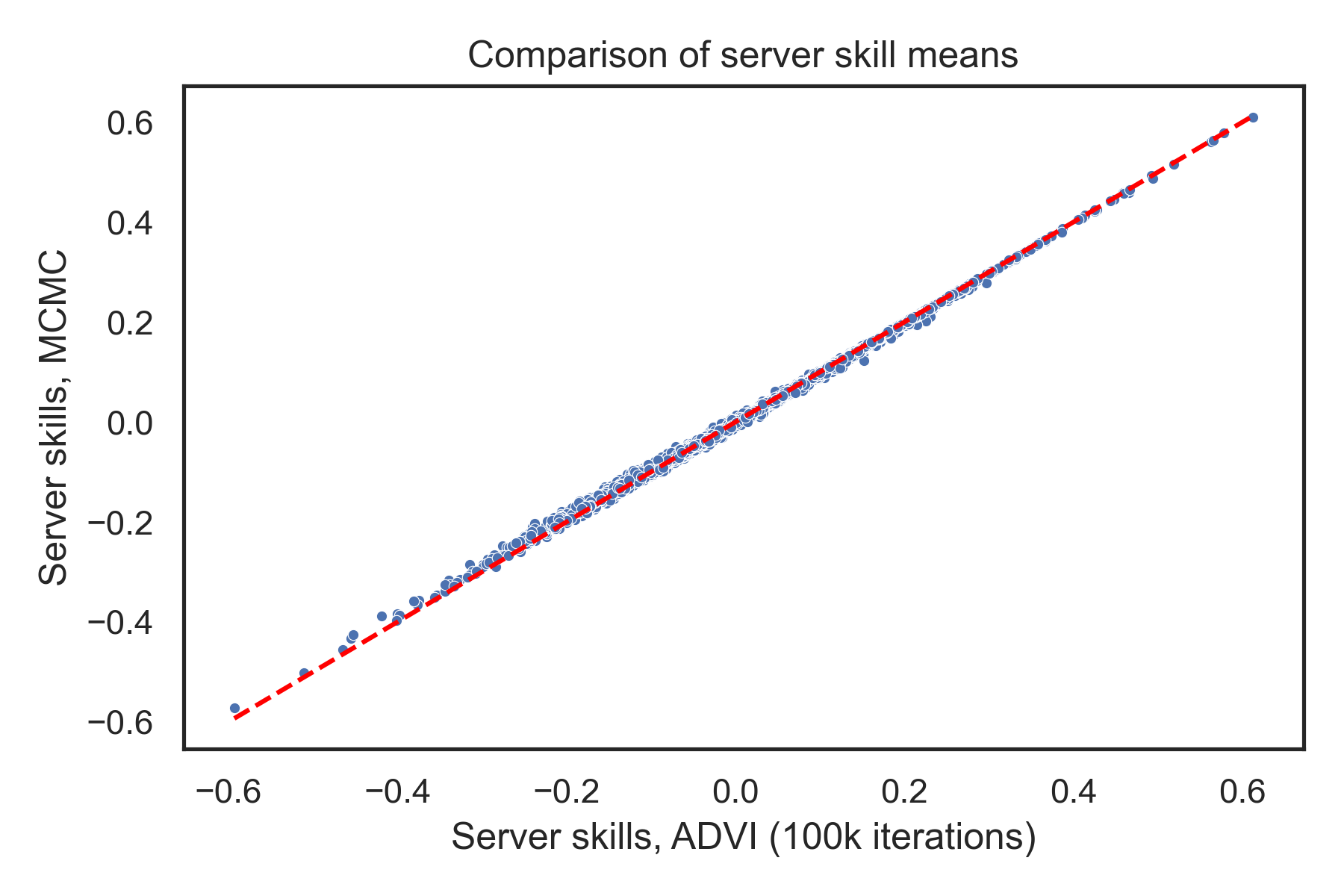
Unfortunately, the convergence criterion doesn’t trigger, so it runs the full 100k iterations. And it takes 12 minutes to do that, so now it’s actually slower than MCMC! On the plus side, the mean estimates look very similar now:

Now, you might protest and say I should have tried running ADVI for some in-between number of steps, and it would have been faster than the sampler and might still have converged. And you’d probably be right! But that’s exactly the problem here: it’s hard to know how many steps you’ll need, and the convergence criterion doesn’t reliably trigger, so it’s not really that helpful. Note that I also tried changing to the absolute option in the convergence criterion, but it didn’t help unfortunately. People are working on improving ADVI’s convergence (e.g. in this paper), but it’s a tricky problem.

Here’s where DADVI can help. While ADVI has a stochastic objective – it estimates its objective with a new random draw at each step – DADVI fixes a set of draws during the optimisation. That introduces some approximation error, but it also means that we can use standard optimizers, which have a clear convergence criterion. So we trade our convergence headaches for a little bit of noise.

To fit DADVI, you can do the following:

from pymc_extras.inference import fit

with m:
	idata_dadvi = fit(method="dadvi")

As you can see, you don’t have to specify a number of steps; it just runs until it detects convergence. It takes about six minutes on my machine, so it’s a fair bit faster than PyMC’s sampler, and it kind of lands in between the short and long ADVI runs. What do the estimates look like?

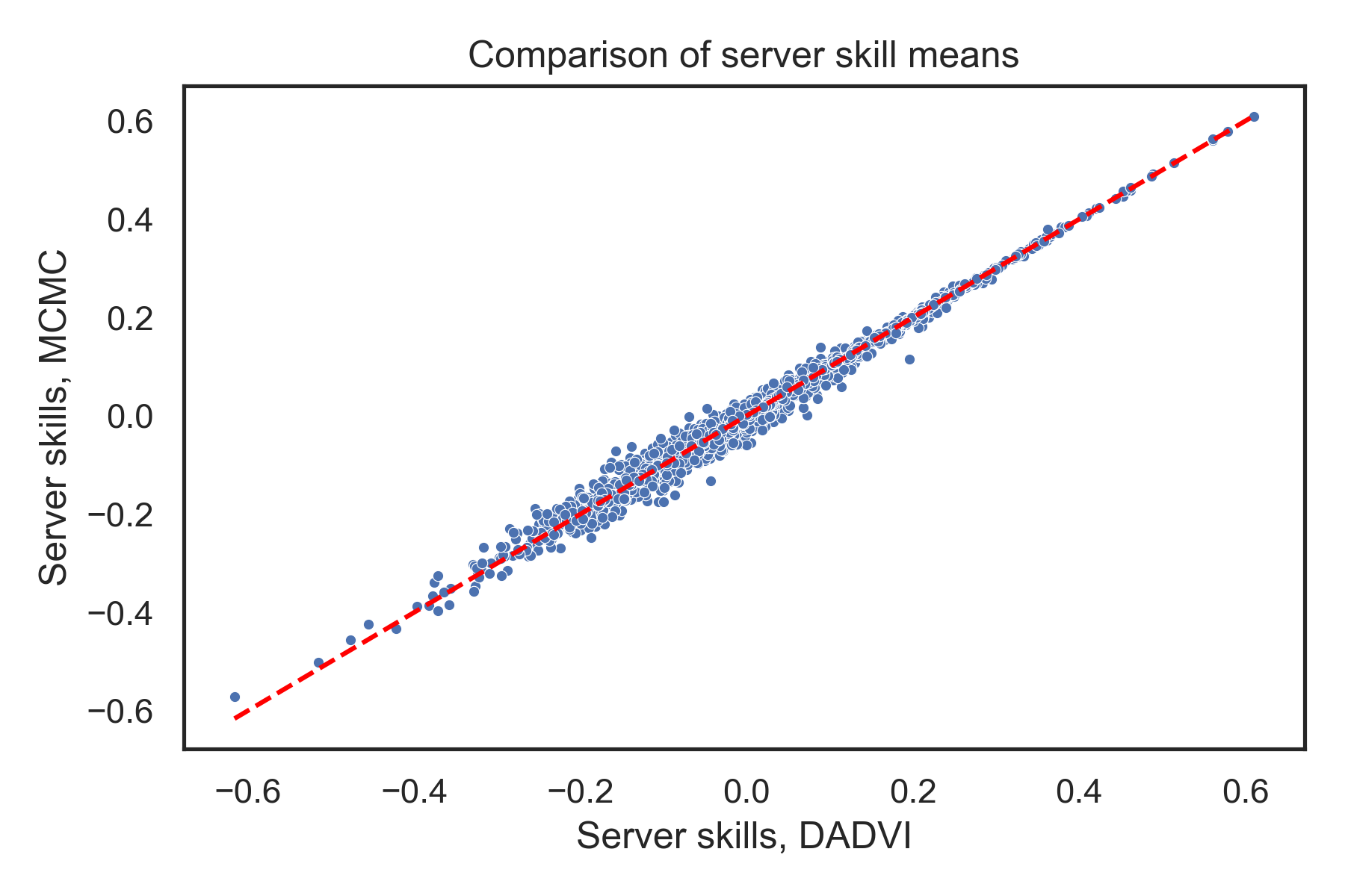
You can see that there is a little bit of scatter introduced by the fixed draws. But as I hope you’ll agree, it’s not that big, and the overall agreement looks pretty good.

We can summarise things by looking at the mean absolute error in the serve and return skill means compared to MCMC, and plotting it against the runtime:

Again, you can see that DADVI comes close to the longer ADVI run in terms of error, but terminates earlier.

Player skill estimates

We can now take a quick look at the mean estimates. We have 2.2k players, but to keep it manageable, I focus on the 25 players with the highest sum of serve and return skills. These should be the best players overall, since the return and serve game are roughly equally important in tennis (you play in each role about half the time). Here they are:

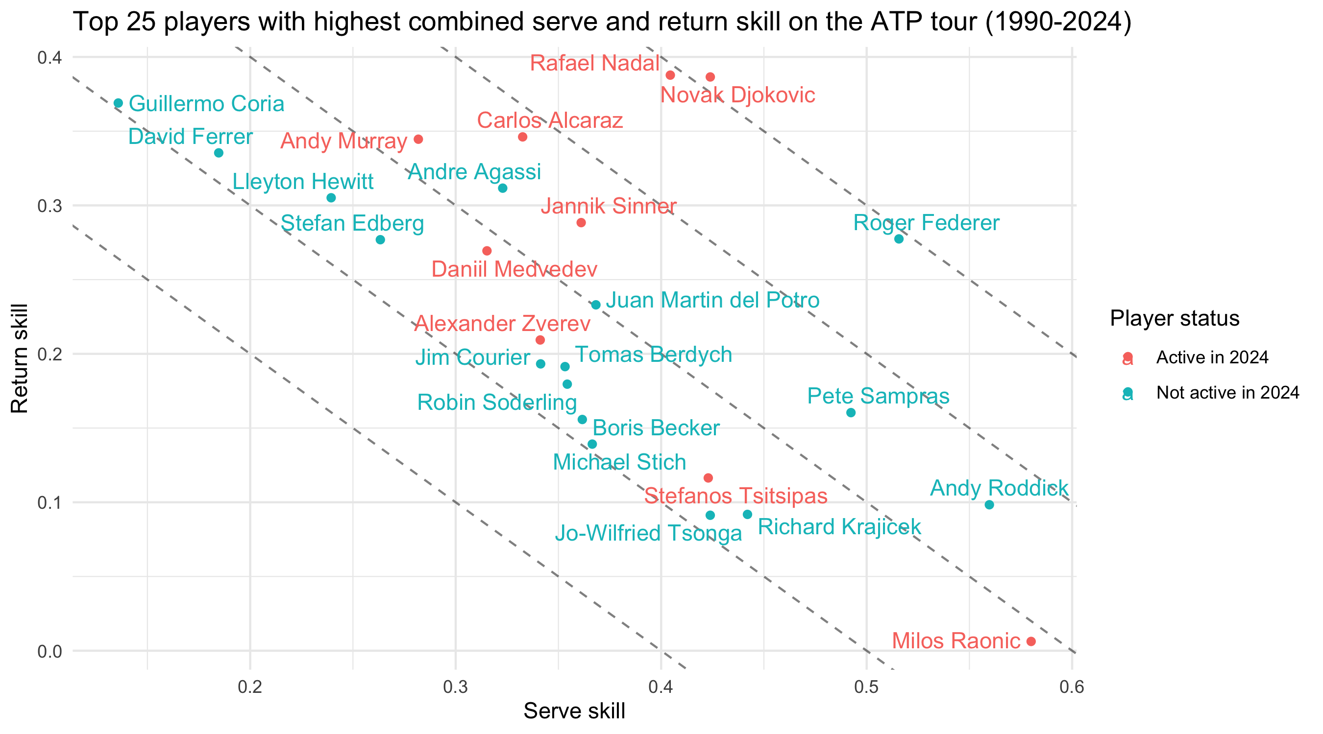
I’ve coloured the points by whether the players were still active in 2024 (some of them have retired by now, so that’s a little bit outdated), which is the last year covered in the dataset. The diagonal lines are lines where the sum of serve and return skills are equal, which you can interpret as the players being roughly equal in strength.

Unfortunately, the dataset doesn’t contain any data for 2025 yet. But I think it’s interesting to see that the big three – Nadal, Djokovic and Federer – sit on or near their own diagonal line with the highest sum of serve and return skills. The new stars, Alcaraz and Sinner, don’t yet quite match their strength, sitting on the next diagonal line down. But note that these are career averages, and Alcaraz and Sinner are still improving, so it’ll be interesting to see how close they can get to the big three as they play more. Their impressive 2025 stats will probably push them closer, and I’m looking forward to checking things again when the dataset is updated.

Summary and thoughts

I hope you enjoyed this little post about DADVI in PyMC, and that it might be useful for your projects. I think the lack of convergence worries does make it more compelling than ADVI, though as I said, I’d like to warn you that there are models where the mean-field objective gets even the means wrong, so it’s best to be a bit cautious. But when the MCMC samplers get too slow, I think DADVI is definitely worth a shot, and I hope you find it useful.

If you want to know more about DADVI, I recommend our paper, which contains lots more detail and theoretical analyses. As I mentioned, I didn’t cover linear response here, which is able to correct the (co-)variances when the means are well estimated, so I’ll cover that in a future blog post when it’s implemented in PyMC. Apart from that, I’d like to investigate how much faster DADVI can run on GPUs (since a fair bit of it can be parallelised).

In the meantime though, if you give DADVI a go, let me know how it goes! And if you want to try to run the model in this post, you can take a look at the code I used here.

Appendix: More model details

If you’re curious, here’s a bit more detail about the tennis model.

I already mentioned that in any given match, we assume that the probability of winning a point on serve, $p$, is a function of the server’s skill and the returner’s skill:

Then, if the server wins $k$ of their $n$ service points, I use a Binomial likelihood:

Note that this assumes that every point on serve is independent and identically distributed, which is a big topic in tennis. In short, it’s not exactly true (there’s some evidence servers tend to do worse when facing break points, for example), but it’s a good approximation a lot of the time.

What makes the model hierarchical is that the serve and return skills are drawn from a prior distribution:

and that these standard deviations, in turn, are drawn from a prior distribution:

I give the intercept a standard normal prior:

You can see that these priors are pretty informative, but they’re reasonable because we know that serve-winning probabilities don’t vary that much from player to player (probably from around 50-80%, if I had to guess).

We can write the model in PyMC as follows:

import pymc as pm

with pm.Model() as m:

	server_skill_sd = pm.HalfNormal("server_sd", sigma=1.0)
	returner_skill_sd = pm.HalfNormal("returner_sd", sigma=1.0)

	server_skills = pm.Normal(
		"server_skills", shape=(n_players,), 
		mu=0.0, sigma=server_skill_sd
	)
	returner_skills = pm.Normal(
		"returner_skills", shape=(n_players,), 
		mu=0.0, sigma=returner_skill_sd
	)

	serve_intercept = pm.Normal("serve_intercept", sigma=1.0)

	pred_logit = (
		server_skills[server_ids] 
		- returner_skills[returner_ids] 
		+ serve_intercept
	)

	likelihood = pm.Binomial(
		"likelihood", logit_p=pred_logit, n=server_out_of, 
		observed=server_won
	)

If you want to know more about how the server_ids, returner_ids etc are derived, you can take a look at the code.